Complete Guide to Quantization and Pruning

Introduction

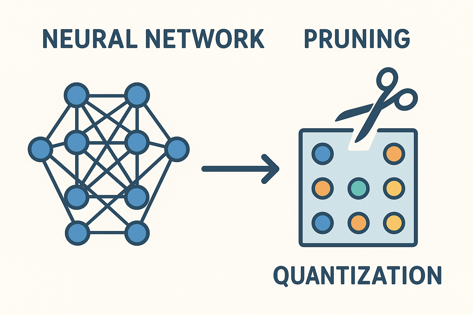
Model compression techniques are essential for deploying deep learning models in resource-constrained environments. Two of the most effective approaches are quantization and pruning, which can significantly reduce model size, memory usage, and inference time while maintaining acceptable performance.

Why Model Compression Matters

Model compression addresses several critical challenges in deep learning deployment:

Key Benefits of Model Compression

Memory Efficiency: Reduced memory footprint enables deployment on mobile devices and edge hardware
Inference Speed: Faster computations through reduced precision arithmetic and fewer operations
Energy Consumption: Lower power requirements for battery-powered devices
Cost Reduction: Decreased cloud computing costs and hardware requirements
Accessibility: Enables AI deployment in environments with limited computational resources

Quantization

Quantization reduces the precision of model weights and activations from floating-point representations (typically 32-bit) to lower-bit representations (8-bit, 4-bit, or even binary).

Fundamentals of Quantization

Uniform Quantization

The most common form maps continuous values to a finite set of discrete levels:

\[Q(x) = \text{round}\left(\frac{x - \text{zero\_point}}{\text{scale}}\right) + \text{zero\_point} \tag{1}\]

Where:

scale: The step size between quantization levels
zero_point: The value that maps to zero in the quantized representation

Asymmetric vs Symmetric Quantization

Symmetric Quantization: Zero point is at the center of the range

Simpler implementation
Better for weights that are roughly centered around zero
Formula: \(Q(x) = \text{round}(x / \text{scale})\)

Asymmetric Quantization: Zero point can be anywhere in the range

Better utilization of the quantization range
More suitable for activations (often non-negative)
Handles skewed distributions better

Types of Quantization

Post-Training Quantization (PTQ)

Quantizes a pre-trained model without retraining:

Static PTQ: Uses a calibration dataset to determine quantization parameters

Faster deployment
No training data required
May have accuracy degradation for complex models

Dynamic PTQ: Determines quantization parameters at runtime

Better accuracy than static PTQ
Slightly higher inference overhead
No calibration dataset needed

Quantization-Aware Training (QAT)

Simulates quantization effects during training:

Higher accuracy preservation
Requires retraining the model
Longer development time but better results

Bit-width Considerations

Table 1: Quantization bit-width comparison

Bit-width	Compression	Accuracy Trade-off	Use Case
8-bit (INT8)	2-4x	Minimal	Most common, well-supported
4-bit	Up to 8x	Moderate	Inference-only scenarios
Binary/Ternary	Up to 32x	Significant	Extreme compression needs

Mixed-Precision Quantization

Different layers use different precisions based on sensitivity analysis:

Critical layers (e.g., first and last layers) kept at higher precision
Less sensitive layers quantized more aggressively
Automated search algorithms determine optimal bit allocation

Pruning

Pruning removes redundant or less important connections, neurons, or entire layers from neural networks.

Types of Pruning

Magnitude-Based Pruning

Removes weights with the smallest absolute values:

Simple to implement
Works well for many architectures
May not capture weight importance accurately

Gradient-Based Pruning

Considers gradients to determine weight importance:

Fisher Information: Uses second-order derivatives
SNIP (Single-shot Network Pruning): Prunes before training
GraSP: Gradient Signal Preservation

Lottery Ticket Hypothesis

Identifies sparse subnetworks that can be trained from scratch:

Iterative magnitude pruning
Rewinding to early training checkpoints
Maintains original network performance

Pruning Granularities

Removes individual weights regardless of their position:

Higher compression ratios possible
Irregular sparsity patterns
May not lead to actual speedup without specialized hardware

Removes entire structures (channels, filters, layers):

Channel Pruning: Removes entire feature map channels
Filter Pruning: Removes convolutional filters
Block Pruning: Removes structured weight blocks

Benefits: - Guaranteed speedup on standard hardware - Maintains regular computation patterns - Easier to implement in existing frameworks

Balances compression and hardware efficiency:

N:M sparsity (e.g., 2:4 sparsity removes 2 out of every 4 weights)
Supported by modern hardware (NVIDIA Ampere architecture)
Good compression with hardware acceleration

Pruning Schedules

flowchart TD
    A[Start Training] --> B{Pruning Strategy}
    B -->|One-Shot| C[Remove All Weights at Once]
    B -->|Gradual| D[Remove Weights Incrementally]
    B -->|Iterative| E[Cycle: Prune-Train-Recover]
    C --> F[Simple Implementation]
    D --> G[Better Accuracy Preservation]
    E --> H[Highest Accuracy Retention]
    F --> I[May Cause Accuracy Drop]
    G --> J[Network Adapts Gradually]
    H --> K[Computationally Expensive]

Advanced Techniques

Knowledge Distillation with Compression

Combines compression with knowledge transfer:

Teacher-student framework during compression
Maintains performance while reducing model size
Particularly effective for quantization

Neural Architecture Search (NAS) for Compression

Automated design of compressed architectures:

Hardware-aware NAS considers deployment constraints
Co-optimization of architecture and compression
Differentiable NAS for quantization

Lottery Ticket Hypothesis Variants

Key Variants

SNIP (Single-shot Network Pruning):

Prunes networks before training
Uses gradient information for importance scoring
Faster than iterative approaches

GraSP (Gradient Signal Preservation):

Maintains gradient flow through the network
Better performance on deep networks
Considers layer-wise interactions

Implementation Examples

PyTorch Quantization Example

import torch
import torch.nn as nn
import torch.quantization as quant

# Define a simple model
class SimpleModel(nn.Module):
    def __init__(self):
        super().__init__()
        self.conv1 = nn.Conv2d(3, 32, 3)
        self.conv2 = nn.Conv2d(32, 64, 3)
        self.fc = nn.Linear(64, 10)
        
    def forward(self, x):
        x = torch.relu(self.conv1(x))
        x = torch.relu(self.conv2(x))
        x = torch.flatten(x, 1)
        x = self.fc(x)
        return x

# Post-training quantization
model = SimpleModel()
model.eval()

# Prepare model for quantization
model.qconfig = quant.get_default_qconfig('fbgemm')
quant.prepare(model, inplace=True)

# Calibrate with sample data
# calibrate_model(model, calibration_data)

# Convert to quantized model
quantized_model = quant.convert(model, inplace=False)

Pruning Example

import torch
import torch.nn.utils.prune as prune

# Apply magnitude-based unstructured pruning
model = SimpleModel()
parameters_to_prune = [
    (model.conv1, 'weight'),
    (model.conv2, 'weight'),
    (model.fc, 'weight'),
]

# Prune 30% of weights globally
prune.global_unstructured(
    parameters_to_prune,
    pruning_method=prune.L1Unstructured,
    amount=0.3,
)

# Make pruning permanent
for module, param in parameters_to_prune:
    prune.remove(module, param)

Structured Pruning Implementation

import torch.nn.utils.prune as prune

def channel_pruning(model, layer_name, amount):
    """Prune channels based on L1 norm of filters"""
    layer = getattr(model, layer_name)
    
    # Calculate channel importance (L1 norm)
    importance = torch.norm(layer.weight.data, p=1, dim=[1, 2, 3])
    
    # Determine channels to prune
    num_channels = len(importance)
    num_prune = int(amount * num_channels)
    
    if num_prune > 0:
        _, indices = torch.topk(importance, num_prune, largest=False)
        
        # Create pruning mask
        prune.structured(layer, name='weight', amount=amount, 
                        dim=0, importance_scores=importance)

# Example usage
channel_pruning(model, 'conv1', 0.5)  # Prune 50% of channels

Best Practices

Quantization Best Practices

Quantization Guidelines

Start with 8-bit quantization: Best balance of compression and accuracy
Use calibration data: Representative of actual deployment data
Layer sensitivity analysis: Identify which layers are most sensitive to quantization
Gradual quantization: Start with less aggressive quantization and increase gradually
Batch normalization folding: Combine BN parameters with preceding layer weights

Pruning Best Practices

Pruning Guidelines

Sensitivity analysis: Determine which layers/channels are most important
Gradual pruning: Remove weights incrementally during training
Fine-tuning: Always fine-tune after pruning to recover accuracy
Layer-wise pruning ratios: Different layers may benefit from different pruning ratios
Structured over unstructured: Choose structured pruning for guaranteed speedup

Combined Approaches

Important Considerations

Order matters: Generally prune first, then quantize
Joint optimization: Consider both techniques simultaneously during training
Hardware considerations: Align compression strategy with deployment hardware
Validation throughout: Monitor accuracy at each compression stage

Tools and Frameworks

Table 2: Model compression tools comparison

Framework	Quantization	Pruning	Special Features
PyTorch	torch.quantization	torch.nn.utils.prune	TorchScript optimization
TensorFlow	Model Optimization Toolkit	Built-in pruning	TFLite for mobile
NVIDIA TensorRT	Automatic mixed precision	Layer fusion	High-performance inference
Intel Neural Compressor	Cross-framework support	Auto-tuning	Hardware-specific optimizations

Specialized Tools

NVIDIA TensorRT:

High-performance inference optimization
Automatic mixed precision
Layer fusion and kernel optimization

Intel Neural Compressor:

Cross-framework quantization
Automatic accuracy-driven tuning
Hardware-specific optimizations

Apache TVM:

Deep learning compiler stack
Auto-tuning for different hardware
Graph-level optimizations

ONNX Runtime:

Cross-platform inference optimization
Dynamic quantization
Graph optimizations

Future Directions

Emerging Quantization Techniques

Mixed-bit Networks: Different precisions for different operations
Learned Quantization: Neural networks learn quantization parameters
Hardware-Software Co-design: Quantization schemes designed for specific hardware

Advanced Pruning Methods

Differentiable Pruning: End-to-end learning of sparse structures
Dynamic Sparsity: Runtime adaptation of sparsity patterns
Cross-layer Dependencies: Pruning decisions considering global network structure

Integration with Other Techniques

graph TD
    A[Model Compression] --> B[Neural Architecture Search]
    A --> C[Federated Learning]
    A --> D[Continual Learning]
    B --> E[Joint Architecture & Compression Optimization]
    C --> F[Compression for Distributed Training]
    D --> G[Maintaining Compression Benefits]

Hardware Considerations

Specialized Accelerators: ASICs designed for sparse and low-precision computation
In-memory Computing: Compression for neuromorphic and analog computing
Edge AI Chips: Dedicated hardware for compressed model inference

Conclusion

Quantization and pruning are essential techniques for practical deep learning deployment. Success requires understanding the trade-offs between compression ratio, accuracy preservation, and hardware compatibility. The field continues to evolve with new methods that push the boundaries of what’s possible with compressed neural networks.

Key Takeaways

Start with well-established techniques (8-bit quantization, magnitude pruning)
Always validate on representative data and deployment hardware
Consider the entire deployment pipeline, not just model accuracy
Combine multiple compression techniques for maximum benefit
Stay informed about hardware-specific optimizations and emerging methods

The future of neural network compression lies in automated, hardware-aware optimization that considers the full spectrum of deployment constraints while maintaining the intelligence and capabilities that make deep learning so powerful.