Active Learning Influence Selection: A Comprehensive Guide

Active Learning Influence Selection: A Comprehensive Guide

Introduction

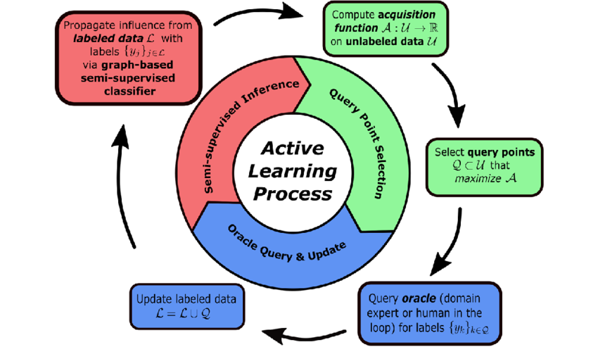
Active learning is a machine learning paradigm where the algorithm can interactively query an oracle (typically a human annotator) to label new data points. The key idea is to select the most informative samples to be labeled, reducing the overall labeling effort while maintaining or improving model performance. This guide focuses on influence selection methods used in active learning strategies.

Table of Contents

1. Fundamentals of Active Learning
2. Influence Selection Strategies
3. Uncertainty-Based Methods
4. Diversity-Based Methods
5. Expected Model Change
6. Expected Error Reduction
7. Influence Functions
8. Query-by-Committee
9. Implementation Considerations
10. Evaluation Metrics
11. Practical Examples
12. Advanced Topics

Fundamentals of Active Learning

The Active Learning Loop

The typical active learning process follows these steps:

1. Start with a small labeled dataset and a large unlabeled pool
2. Train an initial model on the labeled data
3. Apply an influence selection strategy to choose informative samples from the unlabeled pool
4. Get annotations for the selected samples
5. Add the newly labeled samples to the training set
6. Retrain the model and repeat steps 3-6 until a stopping condition is met

Pool-Based vs. Stream-Based Learning

• Pool-based: The learner has access to a pool of unlabeled data and selects the most informative samples
• Stream-based: Samples arrive sequentially, and the learner must decide on-the-fly whether to request labels

Influence Selection Strategies

Influence selection is about identifying which unlabeled samples would be most beneficial to label next. Here are the main strategies:

Uncertainty-Based Methods

These methods select samples that the model is most uncertain about.

Least Confidence

def least_confidence(model, unlabeled_pool, k):
    # Predict probabilities for each sample in the unlabeled pool
    probabilities = model.predict_proba(unlabeled_pool)
    
    # Get the confidence values for the most probable class
    confidences = np.max(probabilities, axis=1)
    
    # Select the k samples with the lowest confidence
    least_confident_indices = np.argsort(confidences)[:k]
    
    return unlabeled_pool[least_confident_indices]

Margin Sampling

Selects samples with the smallest margin between the two most likely classes:

def margin_sampling(model, unlabeled_pool, k):
    # Predict probabilities for each sample in the unlabeled pool
    probabilities = model.predict_proba(unlabeled_pool)
    
    # Sort the probabilities in descending order
    sorted_probs = np.sort(probabilities, axis=1)[:, ::-1]
    
    # Calculate the margin between the first and second most probable classes
    margins = sorted_probs[:, 0] - sorted_probs[:, 1]
    
    # Select the k samples with the smallest margins
    smallest_margin_indices = np.argsort(margins)[:k]
    
    return unlabeled_pool[smallest_margin_indices]

Entropy-Based Sampling

Selects samples with the highest predictive entropy:

def entropy_sampling(model, unlabeled_pool, k):
    # Predict probabilities for each sample in the unlabeled pool
    probabilities = model.predict_proba(unlabeled_pool)
    
    # Calculate entropy for each sample
    entropies = -np.sum(probabilities * np.log(probabilities + 1e-10), axis=1)
    
    # Select the k samples with the highest entropy
    highest_entropy_indices = np.argsort(entropies)[::-1][:k]
    
    return unlabeled_pool[highest_entropy_indices]

Bayesian Active Learning by Disagreement (BALD)

For Bayesian models, BALD selects samples that maximize the mutual information between predictions and model parameters:

def bald_sampling(bayesian_model, unlabeled_pool, k, n_samples=100):
    # Get multiple predictions by sampling from the model's posterior
    probs_samples = []
    for _ in range(n_samples):
        probs = bayesian_model.predict_proba(unlabeled_pool)
        probs_samples.append(probs)
    
    # Stack into a 3D array: (samples, data points, classes)
    probs_samples = np.stack(probs_samples)
    
    # Calculate the average probability across all samples
    mean_probs = np.mean(probs_samples, axis=0)
    
    # Calculate the entropy of the average prediction
    entropy_mean = -np.sum(mean_probs * np.log(mean_probs + 1e-10), axis=1)
    
    # Calculate the average entropy across all samples
    entropy_samples = -np.sum(probs_samples * np.log(probs_samples + 1e-10), axis=2)
    mean_entropy = np.mean(entropy_samples, axis=0)
    
    # Mutual information = entropy of the mean - mean of entropies
    bald_scores = entropy_mean - mean_entropy
    
    # Select the k samples with the highest BALD scores
    highest_bald_indices = np.argsort(bald_scores)[::-1][:k]
    
    return unlabeled_pool[highest_bald_indices]

Diversity-Based Methods

These methods aim to select a diverse set of examples to ensure broad coverage of the input space.

Clustering-Based Sampling

def clustering_based_sampling(unlabeled_pool, k, n_clusters=None):
    if n_clusters is None:
        n_clusters = k
    
    # Apply K-means clustering
    kmeans = KMeans(n_clusters=n_clusters)
    kmeans.fit(unlabeled_pool)
    
    # Get the cluster centers and distances to each point
    centers = kmeans.cluster_centers_
    distances = kmeans.transform(unlabeled_pool)  # Distance to each cluster center
    
    # Select one sample from each cluster (closest to the center)
    selected_indices = []
    for i in range(n_clusters):
        # Get the samples in this cluster
        cluster_samples = np.where(kmeans.labels_ == i)[0]
        
        # Find the sample closest to the center
        closest_sample = cluster_samples[np.argmin(distances[cluster_samples, i])]
        selected_indices.append(closest_sample)
    
    # If we need more samples than clusters, fill with the most uncertain samples
    if k > n_clusters:
        # Implementation depends on uncertainty measure
        pass
    
    return unlabeled_pool[selected_indices[:k]]

Core-Set Approach

The core-set approach aims to select a subset of data that best represents the whole dataset:

def core_set_sampling(labeled_pool, unlabeled_pool, k):
    # Combine labeled and unlabeled data for distance calculations
    all_data = np.vstack((labeled_pool, unlabeled_pool))
    
    # Compute pairwise distances
    distances = pairwise_distances(all_data)
    
    # Split distances into labeled-unlabeled and unlabeled-unlabeled
    n_labeled = labeled_pool.shape[0]
    dist_labeled_unlabeled = distances[:n_labeled, n_labeled:]
    
    # For each unlabeled sample, find the minimum distance to any labeled sample
    min_distances = np.min(dist_labeled_unlabeled, axis=0)
    
    # Select the k samples with the largest minimum distances
    farthest_indices = np.argsort(min_distances)[::-1][:k]
    
    return unlabeled_pool[farthest_indices]

Expected Model Change

The Expected Model Change (EMC) method selects samples that would cause the greatest change in the model if they were labeled:

def expected_model_change(model, unlabeled_pool, k):
    # Predict probabilities for each sample in the unlabeled pool
    probabilities = model.predict_proba(unlabeled_pool)
    n_classes = probabilities.shape[1]
    
    # Calculate expected gradient length for each sample
    expected_changes = []
    for i, x in enumerate(unlabeled_pool):
        # Calculate expected gradient length across all possible labels
        change = 0
        for c in range(n_classes):
            # For each possible class, calculate the gradient if this was the true label
            x_expanded = x.reshape(1, -1)
            # Here we would compute the gradient of the model with respect to the sample
            # For simplicity, we use a placeholder
            gradient = compute_gradient(model, x_expanded, c)
            norm_gradient = np.linalg.norm(gradient)
            
            # Weight by the probability of this class
            change += probabilities[i, c] * norm_gradient
        
        expected_changes.append(change)
    
    # Select the k samples with the highest expected change
    highest_change_indices = np.argsort(expected_changes)[::-1][:k]
    
    return unlabeled_pool[highest_change_indices]

Note: The compute_gradient function would need to be implemented based on the specific model being used.

Expected Error Reduction

The Expected Error Reduction method selects samples that, when labeled, would minimally reduce the model’s expected error:

def expected_error_reduction(model, unlabeled_pool, unlabeled_pool_remaining, k):
    # Predict probabilities for all remaining unlabeled data
    current_probs = model.predict_proba(unlabeled_pool_remaining)
    current_entropy = -np.sum(current_probs * np.log(current_probs + 1e-10), axis=1)
    
    expected_error_reductions = []
    
    # For each sample in the unlabeled pool we're considering
    for i, x in enumerate(unlabeled_pool):
        # Predict probabilities for this sample
        probs = model.predict_proba(x.reshape(1, -1))[0]
        
        # Calculate the expected error reduction for each possible label
        error_reduction = 0
        for c in range(len(probs)):
            # Create a hypothetical new model with this labeled sample
            # For simplicity, we use a placeholder function
            hypothetical_model = train_with_additional_sample(model, x, c)
            
            # Get new probabilities with this model
            new_probs = hypothetical_model.predict_proba(unlabeled_pool_remaining)
            new_entropy = -np.sum(new_probs * np.log(new_probs + 1e-10), axis=1)
            
            # Expected entropy reduction
            reduction = np.sum(current_entropy - new_entropy)
            
            # Weight by the probability of this class
            error_reduction += probs[c] * reduction
        
        expected_error_reductions.append(error_reduction)
    
    # Select the k samples with the highest expected error reduction
    highest_reduction_indices = np.argsort(expected_error_reductions)[::-1][:k]
    
    return unlabeled_pool[highest_reduction_indices]

Note: The train_with_additional_sample function would need to be implemented based on the specific model being used.

Influence Functions

Influence functions approximate the effect of adding or removing a training example without retraining the model:

def influence_function_sampling(model, unlabeled_pool, labeled_pool, k, labels):
    influences = []
    
    # For each unlabeled sample
    for x_u in unlabeled_pool:
        # Calculate the influence of adding this sample to the training set
        influence = calculate_influence(model, x_u, labeled_pool, labels)
        influences.append(influence)
    
    # Select the k samples with the highest influence
    highest_influence_indices = np.argsort(influences)[::-1][:k]
    
    return unlabeled_pool[highest_influence_indices]

Note: The calculate_influence function would need to be implemented based on the specific model and influence metric being used.

Query-by-Committee

Query-by-Committee (QBC) methods train multiple models (a committee) and select samples where they disagree:

def query_by_committee(committee_models, unlabeled_pool, k):
    # Get predictions from all committee members
    all_predictions = []
    for model in committee_models:
        preds = model.predict(unlabeled_pool)
        all_predictions.append(preds)
    
    # Stack predictions into a 2D array (committee members, data points)
    all_predictions = np.stack(all_predictions)
    
    # Calculate disagreement (e.g., using vote entropy)
    disagreements = []
    for i in range(unlabeled_pool.shape[0]):
        # Count votes for each class
        votes = np.bincount(all_predictions[:, i])
        # Normalize to get probabilities
        vote_probs = votes / len(committee_models)
        # Calculate entropy
        entropy = -np.sum(vote_probs * np.log2(vote_probs + 1e-10))
        disagreements.append(entropy)
    
    # Select the k samples with the highest disagreement
    highest_disagreement_indices = np.argsort(disagreements)[::-1][:k]
    
    return unlabeled_pool[highest_disagreement_indices]

Implementation Considerations

Batch Mode Active Learning

In practice, it’s often more efficient to select multiple samples at once. However, simply selecting the top-k samples may lead to redundancy. Consider using:

1. Greedy Selection with Diversity: Select one sample at a time, then update the diversity metrics to avoid selecting similar samples.

def batch_selection_with_diversity(model, unlabeled_pool, k, lambda_diversity=0.5):
    selected_indices = []
    remaining_indices = list(range(len(unlabeled_pool)))
    
    # Calculate uncertainty scores for all samples
    probabilities = model.predict_proba(unlabeled_pool)
    entropies = -np.sum(probabilities * np.log(probabilities + 1e-10), axis=1)
    
    # Calculate distance matrix for diversity
    distance_matrix = pairwise_distances(unlabeled_pool)
    
    for _ in range(k):
        if not remaining_indices:
            break
        
        scores = np.zeros(len(remaining_indices))
        
        # Calculate uncertainty scores
        uncertainty_scores = entropies[remaining_indices]
        
        # Calculate diversity scores (if we have already selected some samples)
        if selected_indices:
            # For each remaining sample, calculate the minimum distance to any selected sample
            diversity_scores = np.min(distance_matrix[remaining_indices][:, selected_indices], axis=1)
        else:
            diversity_scores = np.zeros(len(remaining_indices))
        
        # Normalize scores
        uncertainty_scores = (uncertainty_scores - np.min(uncertainty_scores)) / (np.max(uncertainty_scores) - np.min(uncertainty_scores) + 1e-10)
        if selected_indices:
            diversity_scores = (diversity_scores - np.min(diversity_scores)) / (np.max(diversity_scores) - np.min(diversity_scores) + 1e-10)
        
        # Combine scores
        scores = (1 - lambda_diversity) * uncertainty_scores + lambda_diversity * diversity_scores
        
        # Select the sample with the highest score
        best_idx = np.argmax(scores)
        selected_idx = remaining_indices[best_idx]
        
        # Add to selected and remove from remaining
        selected_indices.append(selected_idx)
        remaining_indices.remove(selected_idx)
    
    return unlabeled_pool[selected_indices]

2. Submodular Function Maximization: Use a submodular function to ensure diversity in the selected batch.

Handling Imbalanced Data

Active learning can inadvertently reinforce class imbalance. Consider:

1. Stratified Sampling: Ensure representation from all classes.
2. Hybrid Approaches: Combine uncertainty-based and density-based methods.
3. Diversity Constraints: Explicitly enforce diversity in feature space.

Computational Efficiency

Some methods (like expected error reduction) can be computationally expensive. Consider:

1. Subsample the Unlabeled Pool: Only consider a random subset for selection.
2. Pre-compute Embeddings: Use a fixed feature extractor to pre-compute embeddings.
3. Approximate Methods: Use approximations for expensive operations.

Evaluation Metrics

Learning Curves

Plot model performance vs. number of labeled samples:

def plot_learning_curve(model_factory, X_train, y_train, X_test, y_test, 
                        active_learning_strategy, initial_size=10, 
                        batch_size=10, n_iterations=20):
    # Initialize with a small labeled set
    labeled_indices = np.random.choice(len(X_train), initial_size, replace=False)
    unlabeled_indices = np.setdiff1d(np.arange(len(X_train)), labeled_indices)
    
    performance = []
    
    for i in range(n_iterations):
        # Create a fresh model
        model = model_factory()
        
        # Train on the currently labeled data
        model.fit(X_train[labeled_indices], y_train[labeled_indices])
        
        # Evaluate on the test set
        score = model.score(X_test, y_test)
        performance.append((len(labeled_indices), score))
        
        # Select the next batch of samples
        if len(unlabeled_indices) > 0:
            # Use the specified active learning strategy
            selected_indices = active_learning_strategy(
                model, X_train[unlabeled_indices], batch_size
            )
            
            # Map back to original indices
            selected_original_indices = unlabeled_indices[selected_indices]
            
            # Update labeled and unlabeled indices
            labeled_indices = np.append(labeled_indices, selected_original_indices)
            unlabeled_indices = np.setdiff1d(unlabeled_indices, selected_original_indices)
    
    # Plot the learning curve
    counts, scores = zip(*performance)
    plt.figure(figsize=(10, 6))
    plt.plot(counts, scores, 'o-')
    plt.xlabel('Number of labeled samples')
    plt.ylabel('Model accuracy')
    plt.title('Active Learning Performance')
    plt.grid(True)
    
    return performance

Comparison with Random Sampling

Always compare your active learning strategy with random sampling as a baseline.

Annotation Efficiency

Calculate how many annotations you saved compared to using the entire dataset.

Practical Examples

Image Classification with Uncertainty Sampling

import numpy as np
from sklearn.datasets import fetch_openml
from sklearn.ensemble import RandomForestClassifier
from sklearn.metrics import accuracy_score
from sklearn.model_selection import train_test_split
import matplotlib.pyplot as plt

# Load data
mnist = fetch_openml('mnist_784', version=1, cache=True)
X, y = mnist['data'], mnist['target']

# Split into train and test
X_train, X_test, y_train, y_test = train_test_split(
    X, y, test_size=0.2, random_state=42
)

# Initially, only a small portion is labeled
initial_size = 100
labeled_indices = np.random.choice(len(X_train), initial_size, replace=False)
unlabeled_indices = np.setdiff1d(np.arange(len(X_train)), labeled_indices)

# Tracking performance
active_learning_performance = []
random_sampling_performance = []

# Active learning loop
for i in range(10):  # 10 iterations
    # Train a model on the currently labeled data
    model = RandomForestClassifier(n_estimators=50, random_state=42)
    model.fit(X_train.iloc[labeled_indices], y_train.iloc[labeled_indices])
    
    # Evaluate on the test set
    y_pred = model.predict(X_test)
    accuracy = accuracy_score(y_test, y_pred)
    active_learning_performance.append((len(labeled_indices), accuracy))
    
    print(f"Iteration {i+1}: {len(labeled_indices)} labeled samples, "
          f"accuracy: {accuracy:.4f}")
    
    # Select 100 new samples using entropy sampling
    if len(unlabeled_indices) > 0:
        # Predict probabilities for each unlabeled sample
        probs = model.predict_proba(X_train.iloc[unlabeled_indices])
        
        # Calculate entropy
        entropies = -np.sum(probs * np.log(probs + 1e-10), axis=1)
        
        # Select samples with the highest entropy
        top_indices = np.argsort(entropies)[::-1][:100]
        
        # Update labeled and unlabeled indices
        selected_indices = unlabeled_indices[top_indices]
        labeled_indices = np.append(labeled_indices, selected_indices)
        unlabeled_indices = np.setdiff1d(unlabeled_indices, selected_indices)

# Plot learning curve
counts, scores = zip(*active_learning_performance)
plt.figure(figsize=(10, 6))
plt.plot(counts, scores, 'o-', label='Active Learning')
plt.xlabel('Number of labeled samples')
plt.ylabel('Model accuracy')
plt.title('Active Learning Performance')
plt.grid(True)
plt.legend()
plt.show()

Iteration 1: 100 labeled samples, accuracy: 0.6917
Iteration 2: 200 labeled samples, accuracy: 0.7290
Iteration 3: 300 labeled samples, accuracy: 0.7716
Iteration 4: 400 labeled samples, accuracy: 0.7817
Iteration 5: 500 labeled samples, accuracy: 0.8239
Iteration 6: 600 labeled samples, accuracy: 0.8227
Iteration 7: 700 labeled samples, accuracy: 0.8282
Iteration 8: 800 labeled samples, accuracy: 0.8435
Iteration 9: 900 labeled samples, accuracy: 0.8454
Iteration 10: 1000 labeled samples, accuracy: 0.8549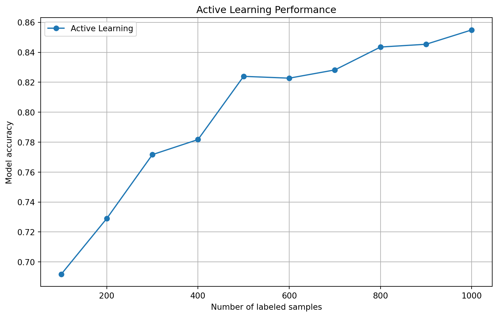

Text Classification with Query-by-Committee

from sklearn.feature_extraction.text import TfidfVectorizer
from sklearn.naive_bayes import MultinomialNB
from sklearn.svm import SVC
from sklearn.ensemble import VotingClassifier
from sklearn.datasets import fetch_20newsgroups

# Load data
categories = ['alt.atheism', 'soc.religion.christian', 'comp.graphics', 'sci.med']
twenty_train = fetch_20newsgroups(subset='train', categories=categories, shuffle=True, random_state=42)
twenty_test = fetch_20newsgroups(subset='test', categories=categories, shuffle=True, random_state=42)

# Feature extraction
vectorizer = TfidfVectorizer(stop_words='english')
X_train = vectorizer.fit_transform(twenty_train.data)
X_test = vectorizer.transform(twenty_test.data)
y_train = twenty_train.target
y_test = twenty_test.target

# Initially, only a small portion is labeled
initial_size = 20
labeled_indices = np.random.choice(len(X_train.toarray()), initial_size, replace=False)
unlabeled_indices = np.setdiff1d(np.arange(len(X_train.toarray())), labeled_indices)

# Create a committee of models
models = [
    ('nb', MultinomialNB()),
    ('svm', SVC(kernel='linear', probability=True)),
    ('svm2', SVC(kernel='rbf', probability=True))
]

# Active learning loop
for i in range(10):  # 10 iterations
    # Train each model on the currently labeled data
    committee_models = []
    for name, model in models:
        model.fit(X_train[labeled_indices], y_train[labeled_indices])
        committee_models.append(model)
    
    # Evaluate using the VotingClassifier
    voting_clf = VotingClassifier(estimators=models, voting='soft')
    voting_clf.fit(X_train[labeled_indices], y_train[labeled_indices])
    
    accuracy = voting_clf.score(X_test, y_test)
    print(f"Iteration {i+1}: {len(labeled_indices)} labeled samples, "
          f"accuracy: {accuracy:.4f}")
    
    # Select 10 new samples using Query-by-Committee
    if len(unlabeled_indices) > 0:
        # Get predictions from all committee members
        all_predictions = []
        for model in committee_models:
            preds = model.predict(X_train[unlabeled_indices])
            all_predictions.append(preds)
        
        # Calculate vote entropy
        vote_entropies = []
        all_predictions = np.array(all_predictions)
        for i in range(len(unlabeled_indices)):
            # Count votes for each class
            votes = np.bincount(all_predictions[:, i], minlength=len(categories))
            # Normalize to get probabilities
            vote_probs = votes / len(committee_models)
            # Calculate entropy
            entropy = -np.sum(vote_probs * np.log2(vote_probs + 1e-10))
            vote_entropies.append(entropy)
        
        # Select samples with the highest vote entropy
        top_indices = np.argsort(vote_entropies)[::-1][:10]
        
        # Update labeled and unlabeled indices
        selected_indices = unlabeled_indices[top_indices]
        labeled_indices = np.append(labeled_indices, selected_indices)
        unlabeled_indices = np.setdiff1d(unlabeled_indices, selected_indices)

Iteration 1: 20 labeled samples, accuracy: 0.2636
Iteration 2: 30 labeled samples, accuracy: 0.3442
Iteration 3: 40 labeled samples, accuracy: 0.3435
Iteration 4: 50 labeled samples, accuracy: 0.4634
Iteration 5: 60 labeled samples, accuracy: 0.5386
Iteration 6: 70 labeled samples, accuracy: 0.5499
Iteration 7: 80 labeled samples, accuracy: 0.6119
Iteration 8: 90 labeled samples, accuracy: 0.6784
Iteration 9: 100 labeled samples, accuracy: 0.7583
Iteration 10: 110 labeled samples, accuracy: 0.7730

Advanced Topics

Transfer Learning with Active Learning

Combining transfer learning with active learning can be powerful:

1. Use pre-trained models as feature extractors.
2. Apply active learning on the feature space.
3. Fine-tune the model on the selected samples.

Active Learning with Deep Learning

Special considerations for deep learning models:

1. Uncertainty Estimation: Use dropout or ensemble methods for better uncertainty estimation.
2. Batch Normalization: Be careful with batch normalization layers when retraining.
3. Data Augmentation: Apply data augmentation to increase the effective size of the labeled pool.

import torch
import torch.nn as nn
import torch.nn.functional as F
from torch.utils.data import DataLoader, Subset
import torchvision.transforms as transforms
import torchvision.datasets as datasets

# Define a simple CNN
class SimpleCNN(nn.Module):
    def __init__(self):
        super(SimpleCNN, self).__init__()
        self.conv1 = nn.Conv2d(1, 32, 3, 1)
        self.conv2 = nn.Conv2d(32, 64, 3, 1)
        self.dropout1 = nn.Dropout2d(0.25)
        self.dropout2 = nn.Dropout2d(0.5)
        self.fc1 = nn.Linear(9216, 128)
        self.fc2 = nn.Linear(128, 10)

    def forward(self, x, dropout=True):
        x = self.conv1(x)
        x = F.relu(x)
        x = self.conv2(x)
        x = F.relu(x)
        x = F.max_pool2d(x, 2)
        if dropout:
            x = self.dropout1(x)
        x = torch.flatten(x, 1)
        x = self.fc1(x)
        x = F.relu(x)
        if dropout:
            x = self.dropout2(x)
        x = self.fc2(x)
        return x

# MC Dropout for uncertainty estimation
def mc_dropout_uncertainty(model, data_loader, n_samples=10):
    model.eval()
    all_probs = []
    
    with torch.no_grad():
        for _ in range(n_samples):
            batch_probs = []
            for data, _ in data_loader:
                output = model(data, dropout=True)
                probs = F.softmax(output, dim=1)
                batch_probs.append(probs)
            
            # Concatenate batch probabilities
            all_probs.append(torch.cat(batch_probs))
    
    # Stack along a new dimension
    all_probs = torch.stack(all_probs)
    
    # Calculate the mean probabilities
    mean_probs = torch.mean(all_probs, dim=0)
    
    # Calculate entropy of the mean prediction
    entropy = -torch.sum(mean_probs * torch.log(mean_probs + 1e-10), dim=1)
    
    return entropy.numpy()

Semi-Supervised Active Learning

Leverage both labeled and unlabeled data during training:

1. Self-Training: Use model predictions on unlabeled data as pseudo-labels.
2. Co-Training: Train multiple models and use their predictions to teach each other.
3. Consistency Regularization: Enforce consistent predictions across different perturbations.

def semi_supervised_active_learning(labeled_X, labeled_y, unlabeled_X, model, confidence_threshold=0.95):
    # Train model on labeled data
    model.fit(labeled_X, labeled_y)
    
    # Predict on unlabeled data
    probabilities = model.predict_proba(unlabeled_X)
    max_probs = np.max(probabilities, axis=1)
    
    # Get high confidence predictions
    confident_indices = np.where(max_probs >= confidence_threshold)[0]
    
    # Get pseudo-labels for confident predictions
    pseudo_labels = model.predict(unlabeled_X[confident_indices])
    
    # Train on combined dataset
    combined_X = np.vstack([labeled_X, unlabeled_X[confident_indices]])
    combined_y = np.concatenate([labeled_y, pseudo_labels])
    
    model.fit(combined_X, combined_y)
    
    return model, confident_indices

Active Learning for Domain Adaptation

When labeled data from the target domain is scarce, active learning can help select the most informative samples:

1. Domain Discrepancy Measures: Select samples that minimize domain discrepancy.
2. Adversarial Selection: Select samples that the domain discriminator is most uncertain about.
3. Feature Space Alignment: Select samples that help align feature spaces between domains.

Human-in-the-Loop Considerations

1. Annotation Interface Design: Make the annotation process intuitive and efficient.
2. Cognitive Load Management: Group similar samples to reduce cognitive switching.
3. Explanations: Provide model explanations to help annotators understand the current model’s decisions.
4. Quality Control: Incorporate mechanisms to detect and correct annotation errors.

Conclusion

Active learning provides a powerful framework for efficiently building machine learning models with limited labeled data. By selecting the most informative samples for annotation, active learning can significantly reduce the labeling effort while maintaining high model performance.

The key to successful active learning is choosing the right influence selection strategy for your specific problem and data characteristics. Consider the following when designing your active learning pipeline:

1. Data Characteristics: Dense vs. sparse data, balanced vs. imbalanced classes, feature distribution.
2. Model Type: Linear models, tree-based models, deep learning models.
3. Computational Resources: Available memory and processing power.
4. Annotation Budget: Number of samples that can be labeled.
5. Task Complexity: Classification vs. regression, number of classes, difficulty of the task.

By carefully considering these factors and implementing the appropriate influence selection methods, you can build high-performance models with minimal annotation effort.