Kolmogorov-Arnold Networks: Revolutionizing Neural Architecture Design

Introduction

Kolmogorov-Arnold Networks (KANs) represent a paradigm shift in neural network architecture design, moving away from the traditional Multi-Layer Perceptron (MLP) approach that has dominated machine learning for decades. Named after mathematicians Andrey Kolmogorov and Vladimir Arnold, these networks are based on the Kolmogorov-Arnold representation theorem, which provides a mathematical foundation for representing multivariate continuous functions.

Unlike traditional neural networks that place fixed activation functions at nodes (neurons), KANs place learnable activation functions on edges (weights). This fundamental architectural change offers several advantages, including better interpretability, higher accuracy with fewer parameters, and improved generalization capabilities.

Mathematical Foundation: The Kolmogorov-Arnold Theorem

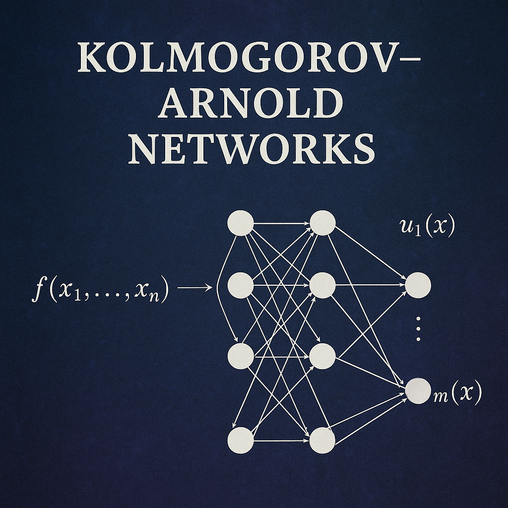
The Kolmogorov-Arnold representation theorem, proven in 1957, states that every multivariate continuous function can be represented as a composition and superposition of continuous functions of a single variable. Mathematically, for any continuous function \(f: [0,1]^n \rightarrow \mathbb{R}\) , there exist continuous functions \(\phi_{q,p}: \mathbb{R} \rightarrow \mathbb{R}\) such that:

\[ f(x_1, x_2, \ldots, x_n) = \sum_{q=0}^{2n} \Phi_q\left( \sum_{p=1}^{n} \phi_{q,p}(x_p) \right) \]

This theorem provides the theoretical foundation for KANs, suggesting that complex multivariate functions can be decomposed into simpler univariate functions arranged in a specific hierarchical structure.

Architecture Overview

Traditional MLPs vs KANs

Traditional MLPs: - Fixed activation functions (ReLU, sigmoid, tanh) at nodes - Linear transformations on edges (weights and biases) - Learning occurs through weight optimization - Limited interpretability due to distributed representations

Kolmogorov-Arnold Networks: - Learnable activation functions on edges - No traditional linear weights - Each edge contains a univariate function (typically B-splines) - Nodes perform simple summation operations - Enhanced interpretability through edge function visualization

KAN Layer Structure

A single KAN layer transforms an input vector of dimension n_in to an output vector of dimension n_out. Each connection between input and output nodes contains a learnable univariate function, typically parameterized using B-splines.

The transformation can be expressed as: \[ y_j = \sum_{i=1}^{n_{\text{in}}} \phi_{i,j}(x_i) \]

Where \(\phi_{i,j}\) represents the learnable function on the edge connecting input i to output j.

Key Components and Implementation

B-Spline Parameterization

KANs typically use B-splines to parameterize the learnable functions on edges. B-splines offer several advantages:

Smoothness: Provide continuous derivatives up to a specified order
Local Support: Changes in one region don’t affect distant regions
Flexibility: Can approximate a wide variety of functions
Computational Efficiency: Enable efficient computation and differentiation

Grid Structure

The B-splines are defined over a grid of control points. Key parameters include:

Grid Size: Number of intervals in the spline grid
Spline Order: Determines smoothness (typically cubic, k=3)
Grid Range: Input domain coverage for the splines

Residual Connections

Modern KAN implementations often include residual connections to improve training stability and enable deeper networks. These connections add a linear component to each edge function:

\[ \phi_{i,j}(x) = \text{spline\_function}(x) + \text{linear\_function}(x) \]

Training Process

Forward Pass

Input Processing: Input features are fed to the first layer
Edge Function Evaluation: Each edge computes its learnable function
Node Summation: Output nodes sum contributions from all incoming edges
Layer Propagation: Process repeats through subsequent layers

Backward Pass

Training KANs requires computing gradients with respect to: - Spline Coefficients: Control points of B-spline functions - Grid Points: Locations of spline knots (in adaptive variants) - Scaling Parameters: Normalization factors for inputs/outputs

Optimization Challenges

Non-convexity: Multiple local minima in the loss landscape
Grid Adaptation: Dynamically adjusting spline grids during training
Regularization: Preventing overfitting in high-capacity edge functions

Advantages of KANs

Enhanced Interpretability

KANs offer superior interpretability compared to traditional MLPs:

Function Visualization: Edge functions can be plotted and analyzed
Feature Attribution: Direct observation of how inputs transform through the network
Symbolic Regression: Potential for discovering analytical expressions

Parameter Efficiency

Despite their flexibility, KANs often achieve better performance with fewer parameters:

Targeted Learning: Functions are learned where needed (on edges)
Shared Complexity: Similar transformations can be learned across different edges
Adaptive Complexity: Grid refinement allows dynamic complexity adjustment

Better Generalization

KANs demonstrate improved generalization capabilities:

Inductive Bias: Architecture naturally incorporates smooth function assumptions
Regularization: B-spline smoothness acts as implicit regularization
Feature Learning: Automatic discovery of relevant transformations

Applications and Use Cases

Scientific Computing

KANs excel in scientific applications where interpretability is crucial:

Physics Modeling: Discovering governing equations from data
Material Science: Property prediction with interpretable relationships
Climate Modeling: Understanding complex environmental interactions

Function Approximation

Natural fit for problems requiring accurate function approximation:

Regression Tasks: Continuous function learning with high accuracy
Time Series: Modeling temporal dependencies with interpretable components
Control Systems: Learning control policies with explainable behavior

Symbolic Regression

KANs can facilitate symbolic regression tasks:

Equation Discovery: Finding analytical expressions for data relationships
Scientific Discovery: Uncovering natural laws from experimental data
Feature Engineering: Automatic discovery of useful feature transformations

Implementation Considerations

Computational Complexity

Memory Requirements: - B-spline coefficients storage - Grid point management - Intermediate activation storage

Computational Cost: - Spline evaluation overhead - Grid adaptation algorithms - Gradient computation complexity

Hyperparameter Tuning

Critical hyperparameters for KANs:

Grid Size: Balance between expressiveness and computational cost
Spline Order: Trade-off between smoothness and flexibility
Network Depth: Number of KAN layers
Width: Number of nodes per layer

Software Implementation

Popular KAN implementations:

PyKAN: Official implementation with comprehensive features
TensorFlow/PyTorch: Custom implementations and third-party libraries
JAX: High-performance implementations for research

Current Limitations and Challenges

Scalability Issues

Memory Overhead: Higher memory requirements compared to MLPs
Training Time: Longer training due to complex function optimization
Large-Scale Applications: Challenges in scaling to very large datasets

Theoretical Gaps

Approximation Theory: Limited theoretical understanding of approximation capabilities
Optimization Landscape: Incomplete analysis of loss surface properties
Generalization Bounds: Lack of theoretical generalization guarantees

Practical Considerations

Implementation Complexity: More complex to implement than standard MLPs
Debugging Difficulty: Harder to diagnose training issues
Limited Tooling: Fewer established best practices and tools

Recent Developments and Research Directions

Architectural Innovations

Multi-dimensional KANs: Extensions to handle tensor inputs directly Convolutional KANs: Integration with convolutional architectures Recurrent KANs: Application to sequential data processing

Optimization Improvements

Adaptive Grids: Dynamic grid refinement during training Regularization Techniques: Novel approaches to prevent overfitting Training Algorithms: Specialized optimizers for KAN training

Application Expansions

Computer Vision: Exploring KANs for image processing tasks Natural Language Processing: Investigating applications in text analysis Reinforcement Learning: Using KANs for policy and value function approximation

Comparison with Other Architectures

KANs vs MLPs

Aspect	KANs	MLPs
Activation Location	Edges	Nodes
Interpretability	High	Low
Parameter Efficiency	Often Better	Standard
Training Complexity	Higher	Lower
Computational Cost	Higher	Lower

KANs vs Transformers

While Transformers excel in sequence modeling, KANs offer advantages in:

Interpretability: Clear function visualization
Scientific Applications: Natural fit for physics-based problems
Small Data Regimes: Better performance with limited training data

KANs vs Decision Trees

Both offer interpretability, but differ in:

Function Types: Continuous vs. piecewise constant
Expressiveness: Higher capacity in KANs
Training: Gradient-based vs. greedy splitting

Future Outlook

Emerging Trends

Hybrid Architectures: Combining KANs with other neural network types Automated Design: Using neural architecture search for KAN optimization Hardware Acceleration: Specialized hardware for efficient KAN computation

Research Opportunities

Theoretical Foundations: Developing rigorous theoretical frameworks Scalability Solutions: Addressing computational and memory challenges Domain-Specific Variants: Tailoring KANs for specific application domains

Industry Adoption

Scientific Software: Integration into computational science tools Interpretable AI: Applications requiring explainable machine learning Edge Computing: Optimized implementations for resource-constrained environments

Conclusion

Kolmogorov-Arnold Networks represent a significant advancement in neural network architecture design, offering a compelling alternative to traditional MLPs. Their foundation in mathematical theory, combined with enhanced interpretability and parameter efficiency, makes them particularly valuable for scientific computing and applications requiring explainable AI.

While challenges remain in terms of computational complexity and scalability, ongoing research continues to address these limitations. As the field matures, KANs are likely to find increased adoption in domains where interpretability and mathematical rigor are paramount.

The future of KANs looks promising, with active research communities working on theoretical foundations, practical implementations, and novel applications. As our understanding of these networks deepens and computational tools improve, KANs may well become a standard tool in the machine learning practitioner’s toolkit.

References and Further Reading

Original KAN Paper: “KAN: Kolmogorov-Arnold Networks” (Liu et al., 2024)
Kolmogorov-Arnold Representation Theorem: Original mathematical foundations
B-Spline Theory: Mathematical background for function parameterization
Scientific Computing Applications: Domain-specific KAN implementations
Interpretable Machine Learning: Broader context for explainable AI methods

This article provides a comprehensive introduction to Kolmogorov-Arnold Networks. For the latest developments and implementations, readers are encouraged to follow recent research publications and open-source projects in the field.