Paper: Learning Transferable Visual Models From Natural Language Supervision Authors: Alec Radford, Jong Wook Kim, Chris Hallacy, Aditya Ramesh, Gabriel Goh, Sandhini Agarwal, Girish Sastry, Amanda Askell, Pamela Mishkin, Jack Clark, Gretchen Krueger, Ilya Sutskever (OpenAI) Submitted: 26 Feb 2021 · arXiv: 2103.00020 · Code/weights: github.com/OpenAI/CLIP Common name: CLIP (Contrastive Language–Image Pre-training)
A note on figures in this guide. The images below are not pixel-for-pixel scans of the original PDF — this environment’s sandbox blocks direct downloads from
arxiv.org, so the original figure bitmaps could not be fetched. Instead, every chart in this guide was regenerated from the exact numeric values reported in the paper’s own text and axis labels (which were extracted successfully), and the one conceptual diagram (Figure 1) was redrawn schematically to match the paper’s description. Tables are transcribed verbatim. Where noted, a small number of details (Sections 7–9 and the appendices) are reconstructed from OpenAI’s companion blog post and well-established secondary coverage of this widely cited paper, since the raw PDF extraction was truncated before reaching those sections.
TL;DR
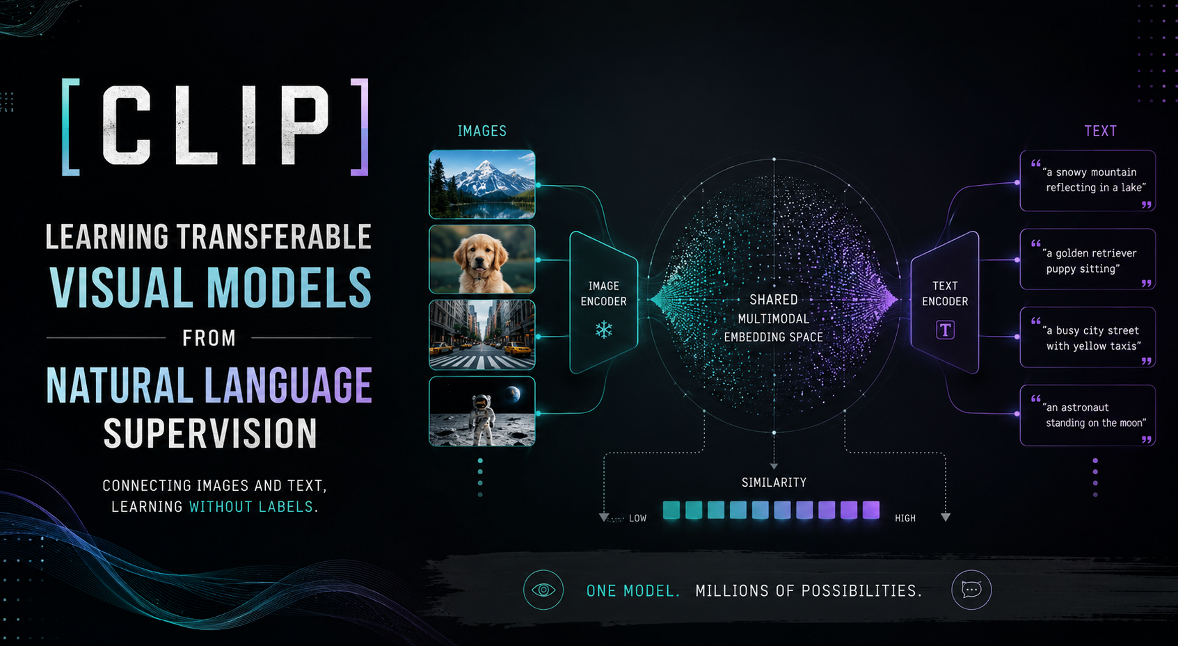
CLIP throws out the idea that a computer vision model must be trained to predict a fixed, hand-labeled list of categories (the “1000 ImageNet classes” paradigm). Instead, it trains an image encoder and a text encoder jointly, from scratch, on 400 million (image, text) pairs scraped from the public internet, using a single proxy task: given a batch of images and a batch of text snippets, figure out which image goes with which text. This is a contrastive objective, not a generative or predictive one — the model never has to generate or reconstruct the exact caption, only to rank the correct pairing above the incorrect ones.
Because the text encoder learns to map arbitrary natural-language descriptions into the same embedding space as images, at test time you can build a classifier for any set of categories just by describing them in words (e.g., “a photo of a dog”, “a photo of a cat”) — no additional labeled training data, no fine-tuning, no new output head. This is what the paper calls zero-shot transfer, and it is CLIP’s central contribution: a single, generically pre-trained model that is benchmarked across more than 30 existing computer vision datasets and is frequently competitive with fully supervised, task-specific baselines. The headline result is that zero-shot CLIP matches the accuracy of the original supervised ResNet-50 on ImageNet without using any of ImageNet’s 1.28 million training labels.
The paper’s contribution is therefore threefold: (a) a dataset-construction and training recipe that makes natural-language supervision computationally practical at scale (400M pairs, contrastive objective, large batch size); (b) an extensive empirical study of zero-shot transfer across dozens of tasks (OCR, action recognition, geo-localization, fine-grained classification); and (c) a careful analysis of what this buys you — better robustness to distribution shift, but still real limitations on abstract/counting tasks, fine-grained tasks, truly out-of-distribution data (e.g., MNIST), and social bias.
Introduction and motivating work
The problem being solved
Standard computer vision pipelines (circa 2021, and still common today) train a model to predict a fixed, predetermined set of object categories — e.g., 1000 ImageNet classes. This has two structural weaknesses:
- Generality: any new visual concept requires new labeled data and, typically, a new output head and a fine-tuning pass.
- Usability: benchmark accuracy on a closed label set is not the same thing as usable, general-purpose visual understanding.
Meanwhile, in NLP, task-agnostic pre-training on raw text (autoregressive and masked language modeling — think GPT-2/GPT-3, BERT, T5) had already demonstrated that web-scale, weakly structured supervision can beat curated, crowd-labeled datasets, and that a single pre-trained model can zero-shot transfer to many downstream tasks via a text-to-text interface. The paper’s motivating question is: can the same “learn directly from raw, uncurated web supervision” recipe work for vision, using text as the supervisory signal instead of labels?
Prior art the paper builds on
The idea of learning visual representations from paired text is not new — the paper is explicit about this lineage:
- Mori et al. (1999): predicting nouns/adjectives in paired documents for content-based image retrieval.
- Quattoni et al. (2007): manifold learning in classifier weight space to predict caption words.
- Srivastava & Salakhutdinov (2012): multimodal Deep Boltzmann Machines over image + text-tag features.
- Joulin et al. (2016): CNNs predicting bag-of-words captions on YFCC100M, competitive with ImageNet pre-training on transfer tasks.
- Li et al. (2017), Visual N-Grams: the first work to zero-shot transfer a generically-trained model to standard image classification benchmarks — but only reaching 11.5% top-1 on ImageNet, far below the fully supervised state of the art (88.4% at the time) and even below classical computer-vision baselines (~50%).
- VirTex (Desai & Johnson, 2020), ICMLM (Bulent Sariyildiz et al., 2020), ConVIRT (Zhang et al., 2020): modern transformer-based approaches (autoregressive, masked-LM, and contrastive objectives respectively) — CLIP is explicitly “a simplified version of ConVIRT trained from scratch.”
Why had this line of work stayed a curiosity rather than a mainstream recipe? Scale. Weakly-supervised approaches that did scale (Mahajan et al., 2018 on Instagram hashtags; Kolesnikov et al., 2019 on JFT-300M) hard-coded a fixed vocabulary of 1,000–18,291 classes and used static softmax classifiers — sacrificing exactly the flexibility that natural language could offer. Meanwhile natural-language approaches like VirTex/ICMLM/ConVIRT trained on only 100k–200k images, “accelerator days” instead of “accelerator years.” CLIP’s contribution is closing this scale gap: 400 million pairs, trained efficiently enough to be practical.
Headline efficiency finding (Figure 2)
Before committing to the final recipe, the authors benchmarked three ways to learn from (image, text) pairs, all measured by zero-shot ImageNet accuracy as a function of the number of images processed:
- A Transformer Language Model that autoregressively predicts the exact caption text (like an image-captioning system) — the weakest and slowest of the three, despite being the most expressive.
- A simpler Bag-of-Words prediction baseline, predicting an unordered bag-of-words encoding of the caption — this alone was 3× more sample-efficient than the transformer LM.
- Bag-of-Words Contrastive (CLIP’s objective) — swapping the predictive objective for a contrastive one on top of the same bag-of-words encoding bought a further 4× efficiency gain.
That 3×-then-4× compounding is the single biggest architectural decision in the paper: don’t try to predict exact words; just distinguish the right pairing from the wrong ones.
The approach
Natural language supervision
The core idea: learn visual representations from the supervisory signal already implicit in natural language paired with images, rather than from a fixed, discretized label taxonomy. Note that different prior papers describe near-identical approaches as “unsupervised,” “self-supervised,” “weakly supervised,” and “supervised” — a sign that the underlying idea (natural language as training signal) is more fundamental than the label people attach to it. The claimed advantages over classic supervised or self-supervised learning:
- Vastly easier to scale — no need for the “1-of-N gold label” annotation format; you can passively harvest supervision from text that already exists on the web.
- Unlike most unsupervised/self-supervised representation learning, it doesn’t just learn a representation — it connects that representation to language, which is what enables flexible zero-shot transfer at the end.
Building a big enough dataset: WIT (WebImageText)
Existing datasets were judged unsuitable at the needed scale:
| Dataset | Size | Issue |
|---|---|---|
| MS-COCO / Visual Genome | ~100K photos each | High quality, crowd-labeled, but far too small |
| YFCC100M | 100M photos | Metadata sparse/noisy; after filtering to only images with natural-language English titles/descriptions, shrinks 6× to ~15M — about ImageNet-sized |
So the authors constructed a new dataset: 400 million (image, text) pairs gathered from a variety of public internet sources. Construction details:
- They searched for pairs whose text includes one of 500,000 queries (base vocabulary = all words occurring ≥100 times in English Wikipedia, augmented with high-PMI bigrams, popular Wikipedia article names, and WordNet synsets).
- Results were approximately class-balanced by including up to 20,000 (image, text) pairs per query.
- Total word count ends up comparable to the WebText dataset used to train GPT-2.
- This dataset is called WIT (WebImageText) — note this predates and is unrelated to Google’s later “WIT: Wikipedia-based Image Text” dataset of the same acronym.
Selecting an efficient pre-training method
Compute is the binding constraint. For context: Mahajan et al. (2018) spent 19 GPU-years; Xie et al. (2020) spent 33 TPUv3-core-years — and those systems only predicted 1,000 ImageNet classes. Learning an open set of visual concepts from raw text looked daunting on cost grounds alone, so training efficiency became the primary criterion for choosing a method (this is the Figure 2 study described above).
The final CLIP objective (contrastive, symmetric, in-batch negatives). Given a batch of N (image, text) pairs, CLIP is trained to predict which of the N × N possible pairings actually occurred. It learns a joint multi-modal embedding space by training an image encoder and text encoder to:
- maximize the cosine similarity of the N correct (image, text) pairs, while
- minimizing the cosine similarity of the N² − N incorrect pairings,
optimized via a symmetric cross-entropy loss over these similarity scores. This batch-construction trick and objective traces back to the multi-class N-pair loss (Sohn, 2016), was popularized as InfoNCE (Oord et al., 2018), and was previously adapted to (text, image) contrastive learning in medical imaging by Zhang et al. (2020) — ConVIRT.
Formalizing the objective
Let \(I_f = f_{\text{image}}(I)\) and \(T_f = f_{\text{text}}(T)\) be the raw encoder outputs for a batch of \(N\) images and \(N\) texts. Project each into a shared \(d_e\)-dimensional embedding space via learned linear maps \(W_i\) and \(W_t\), then L2-normalize:
\[ I_e = \frac{I_f W_i}{\lVert I_f W_i \rVert_2}, \qquad T_e = \frac{T_f W_t}{\lVert T_f W_t \rVert_2} \]
Compute the scaled pairwise cosine-similarity (“logits”) matrix using a learned temperature \(t\):
\[ \text{logits}_{jk} = \left(I_e T_e^{\top}\right)_{jk} \cdot e^{t}, \qquad j,k \in \{1, \dots, N\} \]
The loss is the average of two cross-entropy terms — one that, for each image row, treats the matching text as the correct class among all \(N\) texts in the batch; and one that does the same for each text column against all \(N\) images:
\[ \mathcal{L} = \frac{1}{2}\Big( \underbrace{\text{CE}(\text{logits}, \; \mathbf{y} \mid \text{rows})}_{\text{image} \rightarrow \text{text}} \;+\; \underbrace{\text{CE}(\text{logits}^{\top}, \; \mathbf{y} \mid \text{rows})}_{\text{text} \rightarrow \text{image}} \Big), \qquad \mathbf{y} = [0, 1, \dots, N-1] \]
i.e. the ground-truth label for row/column \(k\) is simply \(k\) itself — the diagonal of the \(N \times N\) similarity matrix should dominate.
Official pseudocode (Figure 3, transcribed verbatim)
# image_encoder - ResNet or Vision Transformer
# text_encoder   - CBOW or Text Transformer
# I[n, h, w, c]  - minibatch of aligned images
# T[n, l]        - minibatch of aligned texts
# W_i[d_i, d_e]  - learned proj of image to embed
# W_t[d_t, d_e]  - learned proj of text to embed
# t              - learned temperature parameter

# extract feature representations of each modality
I_f = image_encoder(I)          # [n, d_i]
T_f = text_encoder(T)           # [n, d_t]

# joint multimodal embedding [n, d_e]
I_e = l2_normalize(np.dot(I_f, W_i), axis=1)
T_e = l2_normalize(np.dot(T_f, W_t), axis=1)

# scaled pairwise cosine similarities [n, n]
logits = np.dot(I_e, T_e.T) * np.exp(t)

# symmetric loss function
labels = np.arange(n)
loss_i = cross_entropy_loss(logits, labels, axis=0)
loss_t = cross_entropy_loss(logits, labels, axis=1)
loss   = (loss_i + loss_t) / 2
Design simplifications relative to ConVIRT
Because the 400M-pair dataset makes over-fitting a non-issue, the authors simplified training considerably versus Zhang et al. (2020):
- Trained entirely from scratch — no ImageNet-pretrained image encoder, no pretrained text encoder.
- No non-linear projection head between encoder representation and the shared embedding space (a technique introduced by Bachman et al., 2019, popularized by Chen et al., 2020b / SimCLR) — CLIP uses only a linear projection per modality, with no observed efficiency loss.
- No random sentence sampling transformation — most WIT captions are already a single sentence.
- Minimal image augmentation — just a random square crop from a resized image.
- The temperature \(\tau\) is a learned parameter (log-parameterized multiplicative scalar), not a manually-tuned hyperparameter, initialized equivalent to 0.07 (Wu et al., 2018) and clipped to prevent the logits from being scaled by more than 100 (needed for training stability).
Model architecture
Two families of image encoder were trained:
- ResNet-50, with several modifications: ResNet-D improvements (He et al., 2019), antialiased rect-2 blur pooling (Zhang, 2019), and — notably — the global average pooling layer is replaced by an attention-pooling mechanism: a single layer of transformer-style multi-head QKV attention where the query is conditioned on the global-average-pooled image representation.
- Vision Transformer (ViT) (Dosovitskiy et al., 2020), followed closely, with a minor tweak: an extra layer norm applied to the combined patch + position embeddings before the transformer, and a slightly different initialization.
Text encoder: a Transformer (Vaswani et al., 2017) using the architectural modifications of Radford et al. (2019) — i.e., GPT-2-style. Base configuration: 63M parameters, 12 layers, 512-wide, 8 attention heads, operating over a lower-cased byte-pair encoding (BPE) vocabulary of 49,152 tokens (Sennrich et al., 2015), with max sequence length capped at 76 for efficiency. Text is bracketed with [SOS]/[EOS] tokens; the [EOS] activation at the top layer is layer-normalized and linearly projected into the shared embedding space. Masked self-attention is retained (even though not strictly required for a contrastive-only objective) to preserve the option of initializing from, or jointly training with, a language-modeling objective in future work.
Scaling rule: rather than scaling only width (as in Mahajan et al., 2018) or only depth (as in the original ResNet paper), the image encoder is scaled the way EfficientNet scales (Tan & Le, 2019) — jointly across width, depth, and resolution — though CLIP uses a simple equal allocation across the three dimensions rather than EfficientNet’s tuned ratio. The text encoder is scaled in width only, proportionally to the ResNet’s width increase, with no depth scaling — the paper found CLIP’s performance much less sensitive to text-encoder capacity than to image-encoder capacity.
Training configuration
| Setting | Value |
|---|---|
| Models trained | 5 ResNets (RN50, RN101, RN50x4, RN50x16, RN50x64 at ~4×/16×/64× RN50 compute) + 3 ViTs (ViT-B/32, ViT-B/16, ViT-L/14) |
| Epochs | 32 |
| Optimizer | Adam, with decoupled weight decay (AdamW-style, Loshchilov & Hutter, 2017), applied to all weights except gains/biases |
| LR schedule | Cosine decay (Loshchilov & Hutter, 2016) |
| Hyperparameter search | Grid + random search + manual tuning on RN50 @ 1 epoch, then heuristically adapted for larger models |
| Temperature \(\tau\) | Learned; init ≈ 0.07; clipped to cap logit scaling at 100× |
| Batch size | 32,768 (very large) |
| Precision / memory tricks | Mixed precision, gradient checkpointing, half-precision Adam statistics, half-precision stochastically-rounded text-encoder weights, sharded embedding-similarity computation across GPUs |
| Largest ResNet (RN50x64) | 18 days on 592 V100 GPUs |
| Largest ViT (ViT-L/14) | 12 days on 256 V100 GPUs |
| Best model | ViT-L/14, further pre-trained 1 extra epoch at 336px resolution (FixRes-style, Touvron et al., 2019) — denoted ViT-L/14@336px. Unless stated otherwise, “CLIP” in the paper’s results refers to this model. |
Recreated overview diagram
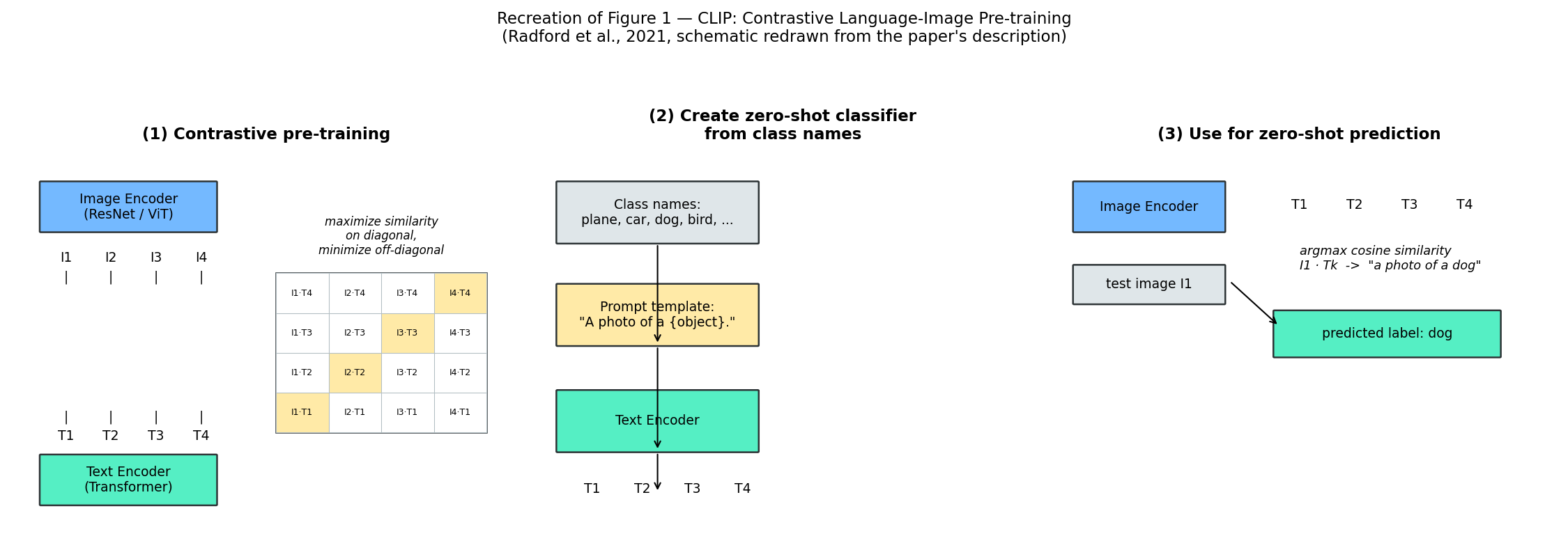
Reading the three panels: (1) during pre-training, an image encoder and text encoder are jointly trained so that the cosine similarity of matched image/text embeddings (\(I_k \cdot T_k\), the diagonal) is high and mismatched pairs are low. (2) at evaluation time, the class names of a brand-new target dataset (e.g. “plane”, “car”, “dog”, “bird”) are wrapped in a prompt template like “A photo of a {object}.” and pushed through the (frozen) text encoder — this produces one embedding vector per class, which functions as the weight vector of a linear classifier synthesized entirely from language. (3) for a new test image, its embedding is compared against every class’s text embedding, and the class with the highest cosine similarity is the zero-shot prediction. This third step is why the paper describes the text encoder as a hypernetwork (Ha et al., 2016): a network that generates the weights of another network (here, a linear classifier) instead of computing the target quantity itself. The idea of zero-shot classifiers of this exact form (compare image embedding to embeddings of natural-language class descriptions) traces back to Lei Ba et al. (2015) and, for language-generated classifiers specifically, Elhoseiny et al. (2013).
Experiments
Zero-shot transfer
What “zero-shot” means here
The paper deliberately broadens “zero-shot learning” beyond its usual computer-vision meaning (generalizing to unseen categories) to mean generalizing to unseen datasets/distributions — motivated by Larochelle et al. (2008)’s zero-data learning framing. The authors argue this is really a proxy for measuring task-learning capability, not just representation quality: many popular CV benchmarks (CIFAR-10, for instance) were built as generic-method testbeds rather than as measurements of one specific real-world task, so zero-shot transfer to them is best read as a test of robustness/generalization, which the paper revisits directly in the robustness section below.
Mechanics of zero-shot classification
For a target dataset, embed every class name (through the frozen text encoder) once, embed the test image once, compute cosine similarities, scale by the learned temperature \(\tau\), and softmax to get a probability distribution. This is literally a multinomial logistic regression classifier with L2-normalized inputs, L2-normalized weights, no bias term, and temperature scaling — except the weights were “written” by the text encoder rather than learned by gradient descent on that specific task. Framed this way, every step of CLIP pre-training is optimizing performance on a randomly-constructed proxy classification problem with 1 example per class and 32,768 total classes (the batch size). Since the zero-shot classifier only needs to be computed once per dataset, its cost is amortized across every prediction made on that dataset.
Initial comparison to Visual N-Grams (Table 1)
| Dataset | Visual N-Grams | CLIP |
|---|---|---|
| aYahoo | 72.4 | 98.4 |
| ImageNet | 11.5 | 76.2 |
| SUN | 23.0 | 58.5 |
The authors are careful to caveat that this is contextualizing, not a controlled ablation: CLIP trains on 10× more data, uses an image encoder needing ~100× more compute per prediction, and likely uses over 1000× more total training compute than Visual N-Grams — plus a transformer architecture that didn’t exist in 2017. As a fairer, closer comparison, they trained a CLIP ResNet-50 on the exact same YFCC100M dataset Visual N-Grams used, and matched its reported ImageNet performance within a single V100 GPU-day.
CLIP’s ImageNet result (76.2%) matches the original supervised ResNet-50’s accuracy — without using any of the 1.28 million labeled ImageNet training images. Top-5 accuracy reaches 95%, matching Inception-v4.
Prompt engineering and ensembling (Figure 4)
Two subtle but consequential engineering choices:
- Polysemy is a real problem. Bare class names lack context — e.g., ImageNet’s “crane” could mean the bird or the construction equipment; Oxford-IIIT Pets’ “boxer” could mean the dog breed or the athlete.
- The pre-training distribution is mostly full sentences, not bare words. Using the template “A photo of a {label}.” as a default closes this distribution gap and alone improves ImageNet accuracy by 1.3%.
- Dataset-specific prompt customization helps further: “A photo of a {label}, a type of pet.” for Oxford-IIIT Pets; specifying food/aircraft for Food101/FGVCAircraft; quoting the text/number for OCR datasets; “a satellite photo of a {label}.” for satellite imagery.
- Ensembling across many prompt templates (e.g., “a photo of a big {label}”, “a photo of a small {label}”) in embedding space (not probability space) — this means a single cached, averaged text embedding per class captures the whole ensemble at no extra inference cost. On ImageNet, ensembling 80 different prompts contributes an additional 3.5%.
- Combined effect: prompt engineering + ensembling together improve ImageNet accuracy by almost 5%, at essentially zero marginal inference cost once amortized — described in the paper as equivalent to roughly a 4× compute gain, but “free.”
Zero-shot CLIP vs. a fully supervised linear probe on ResNet-50 (Figure 5)
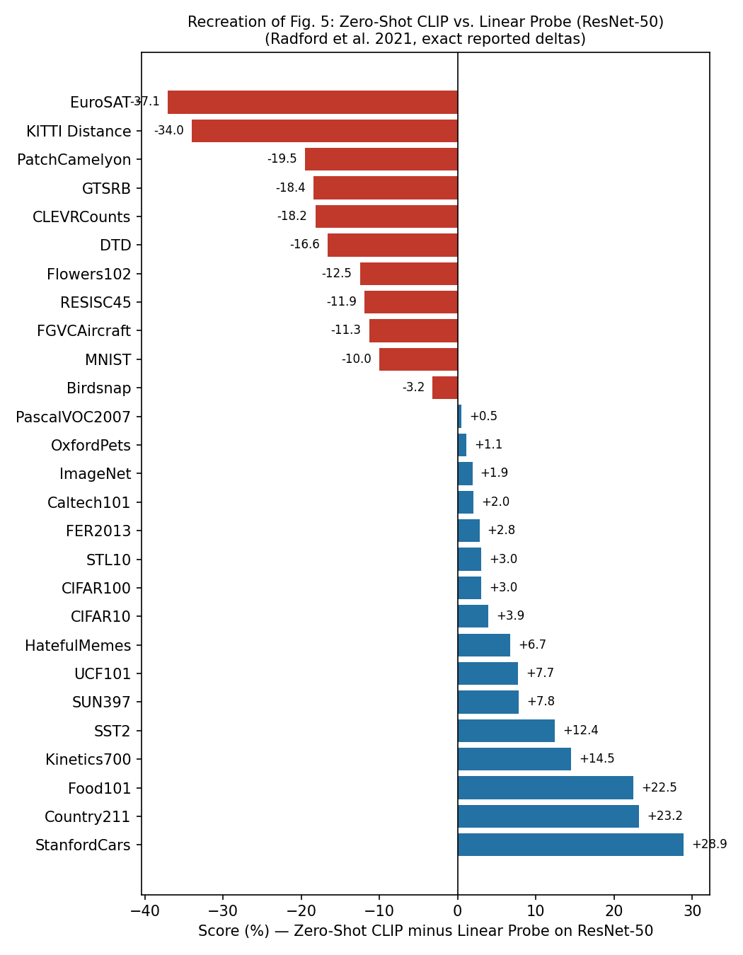
Zero-shot CLIP wins on 16 of 27 datasets, including ImageNet itself (+1.9). Patterns worth noting:
- General object classification (ImageNet, CIFAR-10/100, STL-10, PascalVOC2007): CLIP is roughly on par or slightly ahead. On STL-10, CLIP hits 99.3%, a new state of the art at the time — with zero training examples.
- Action recognition in video (Kinetics700 +14.5, UCF101 +7.7): CLIP does markedly better, hypothesized to be because natural language supervises verbs/actions more broadly than ImageNet’s noun-centric labels.
- Weakest spots: EuroSAT (−37.1), KITTI Distance (−34.0), PatchCamelyon (−19.5), GTSRB (−18.4), CLEVRCounts (−18.2) — specialized, abstract, or synthetic tasks (satellite classification, distance estimation, tumor detection, traffic-sign recognition, counting) where CLIP’s web-scraped pre-training data offers little natural coverage.
Zero-shot vs. few-shot (Figures 6–8)
- Zero-shot CLIP matches the average performance of a 4-shot linear classifier trained on the same CLIP feature space, and nearly matches a 16-shot classifier’s performance across the broader evaluation suite (Figure 6). This is notable because normally you’d expect some labeled data to always help — the paper’s explanation is that CLIP’s zero-shot classifier is directly specified via language, whereas example-based (few-shot) learning must infer the intended concept indirectly from images, and a single image often contains many entangled visual concepts (background, pose, lighting, etc.), which is especially unreliable in the 1-shot regime.
- Effective data efficiency varies enormously by dataset (Figure 7, below): from under 1 labeled example per class (Flowers102, EuroSAT — where zero-shot already beats a 1-shot linear probe) up to an estimated 184 examples per class (FER2013). Median 5.4, mean 20.8 examples/class across the 26 datasets studied.
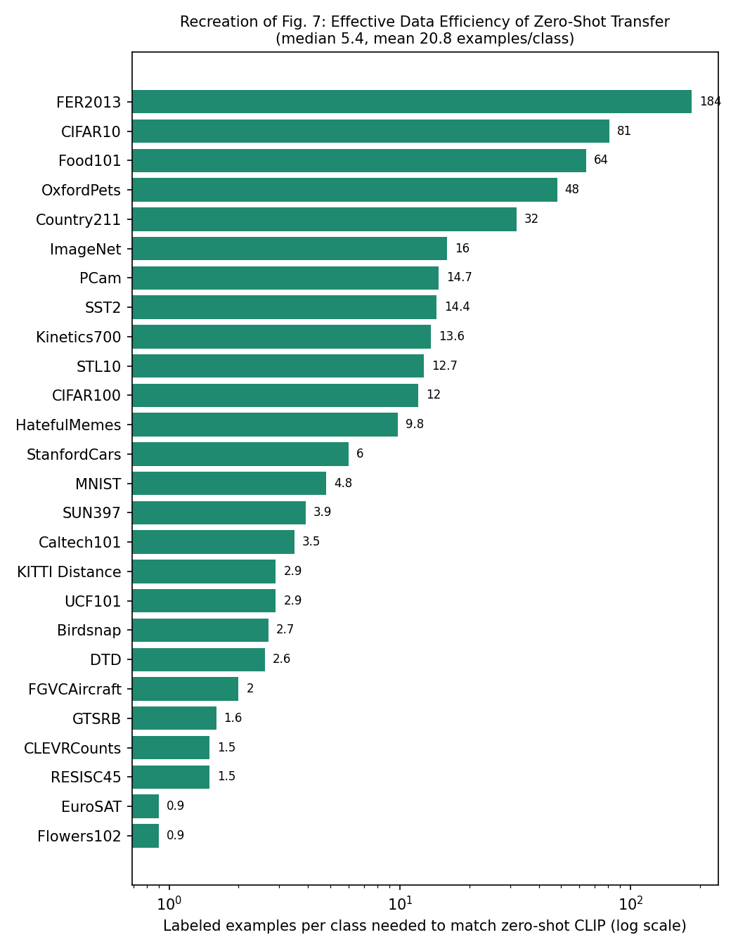
- Because zero-shot CLIP is itself effectively a linear classifier, fully-supervised linear-probe performance roughly upper-bounds what zero-shot transfer can achieve (Figure 8 in the original paper). Across datasets there is a strong correlation (\(r = 0.82\), \(p < 10^{-6}\)) between zero-shot and fully-supervised linear-probe accuracy, but zero-shot typically trails by 10–25 points; only 5 datasets (STL-10, CIFAR-10, Food101, OxfordPets, Caltech101 — all already >90% for both) come within 3 points of the supervised ceiling.
- Scaling behaviour (Figure 9 in the original paper): average zero-shot error across 39 evaluations on 36 datasets follows a smooth log-log linear trend as a function of model compute, across a 44× range of compute spanning the 5 ResNet-family CLIP models — echoing the compute-scaling laws documented for GPT-family models (Kaplan et al., 2020). Individual per-task curves are much noisier than the aggregate trend.
Representation learning (linear-probe evaluation)
Rather than end-to-end fine-tuning (which the authors note can mask failures of the pre-training representation itself, since fine-tuning adapts the representation per-dataset), the paper deliberately evaluates via linear probes: fit a linear classifier on top of frozen features and measure accuracy. This choice also mirrors the zero-shot evaluation methodology, enabling apples-to-apples comparison, and keeps the study of 66 models × 27 datasets (1,782 evaluations) computationally tractable and free of confounding hyperparameter-tuning effort.
Findings (Figure 10 in the original paper):
- On the standardized 12-dataset suite of Kornblith et al. (2019): small CLIP ResNets beat other ImageNet-1K-trained ResNets (including BiT-S) but underperform ImageNet-21K-trained BiT-M and EfficientNet-family models at similar compute.
- But CLIP scales exceptionally well: the largest ResNet trained (RN50x64) slightly outperforms the best existing public model (Noisy Student EfficientNet-L2) on both overall score and compute efficiency, on this 12-dataset suite.
- CLIP Vision Transformers are ~3× more compute-efficient than CLIP ResNets — echoing Dosovitskiy et al. (2020)’s original ViT-vs-CNN efficiency finding, now shown to hold for CLIP’s contrastive training too.
- The single best CLIP model (ViT-L/14@336px) beats the best existing model by an average of 2.6% on the 12-dataset suite.
- On the broader, 27-dataset suite (chosen partly to include tasks like geo-localization, OCR, facial-emotion recognition, and action recognition that Kornblith et al.’s 12-dataset suite entirely misses — arguably a selection bias toward ImageNet-adjacent tasks), every CLIP model, at every scale, is more compute-efficient than every other system evaluated, and the best-model improvement margin widens to 5%.
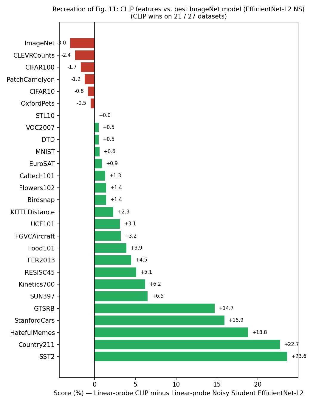
CLIP’s features beat the best public ImageNet model (Noisy Student EfficientNet-L2) on 21 of 27 datasets — with the largest gains on OCR-flavored tasks (SST2 +23.6, HatefulMemes +18.8), geo-localization/scene recognition (Country211 +22.7, SUN397 +6.5), and fine-grained car/traffic-sign recognition (StanfordCars +15.9, GTSRB +14.7 — the authors suggest ImageNet’s single “street/traffic sign” label collapses intra-class detail that hurts fine-grained transfer). CLIP loses, unsurprisingly, on ImageNet itself (−3.0, the dataset EfficientNet was directly trained on) and on low-resolution CIFAR-10/100 (likely due to CLIP’s lack of scale-based data augmentation).
Robustness to natural distribution shift
Background: Since ~2015, “superhuman” ImageNet accuracy claims have repeatedly failed to hold up once models are tested on natural distribution shifts (as opposed to synthetic corruptions like ImageNet-C or adversarial perturbations). Taori et al. (2020) formalized this with 7 natural-shift test sets — ImageNetV2, ImageNet Sketch, Youtube-BB, ImageNet-Vid, ObjectNet, ImageNet-A, ImageNet-R — and the concept of effective robustness (accuracy gain under shift beyond what’s predicted by in-distribution accuracy alone) versus mere relative robustness (any accuracy gain at all under shift).
Key finding: a ResNet-101 matched to CLIP’s zero-shot ImageNet accuracy (76.2%) makes far more mistakes under natural distribution shift than zero-shot CLIP does. Zero-shot CLIP shrinks the “effective robustness gap” (the gap between ImageNet accuracy and shifted-distribution accuracy) by up to 75%.
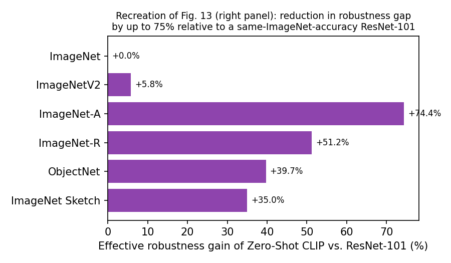
But adapting CLIP to ImageNet erodes this benefit. Fitting an L2-regularized logistic-regression classifier on CLIP features using the ImageNet training set raises ImageNet accuracy by +9.2% (to 85.4%, tying 2018’s SOTA) — yet average accuracy under distribution shift barely moves, and actually drops on ImageNet-R (−4.7), ObjectNet (−3.8), ImageNet Sketch (−2.8), and ImageNet-A (−1.9). Only ImageNetV2 improves substantially (+5.8), which the authors attribute to ImageNetV2 having been collected via a process almost identical to the original ImageNet’s. In other words: a 9.2-point, “3 years of SOTA progress”-sized jump in ImageNet accuracy buys essentially nothing in real-world robustness — a striking illustration of Goodhart’s-law-style benchmark overfitting.
A second robustness intervention — generating a custom zero-shot classifier per evaluation dataset (rather than reusing/pooling a fixed 1000-way ImageNet classifier, which Taori et al. had to do via class-hierarchy max-pooling for datasets like Youtube-BB and ImageNet-Vid whose classes are ImageNet superclasses) — improves average effective robustness by another 5%, concentrated in large gains on the few datasets where class granularity actually differed from ImageNet’s.
The paper also traces the zero-shot → few-shot → fully-supervised continuum (Figure 15 in the original): higher effective robustness correlates with less distribution-specific training data used, and this benefit erodes steadily as more labeled ImageNet examples are used to adapt the classifier, disappearing almost entirely by full supervision.
Comparison to human performance
To contextualize task difficulty, five humans each labeled all 3,669 test images of Oxford-IIIT Pets (37 cat/dog breeds), in zero-shot, one-shot, and two-shot settings (with the “shots” being example images per breed, no internet lookups allowed).
| Setting | Accuracy (full dataset) | Majority vote | Accuracy (on guesses only) | Majority vote (on guesses) |
|---|---|---|---|---|
| Zero-shot human | 53.7 | 57.0 | 69.7 | 63.9 |
| Zero-shot CLIP | 93.5 | 93.5 | 93.5 | 93.5 |
| One-shot human | 75.7 | 80.3 | 78.5 | 81.2 |
| Two-shot human | 75.7 | 85.0 | 79.2 | 86.1 |
The striking pattern: humans jump from 54% → 76% accuracy after just one example per class, with almost all of that gain concentrated in images the human was previously uncertain about — i.e., humans “know what they don’t know” and can resolve that uncertainty from a single example. CLIP’s few-shot methods show no such jump (in fact, the paper notes few-shot linear probes on CLIP features can underperform zero-shot CLIP, a counter-intuitive result revisited in the Limitations section). This exposes a real gap between human sample-efficient learning (which appears to integrate strong priors) and current few-shot machine learning methods, which mostly do not make effective use of prior knowledge. The hardest classes for CLIP also tend to be the hardest for humans, suggesting shared sources of difficulty — likely label noise and genuinely out-of-distribution or ambiguous images.
Data overlap analysis
A natural worry with a 400M-image internet-scraped pre-training set: some evaluation-set images might have leaked into training, inflating reported zero-shot accuracy. Rather than trying to scrub all possible overlaps up front (which would require knowing every future eval dataset in advance, and would make adding new evals expensive), the authors instead measured and quantified the effect:
- Run a duplicate detector (detailed in the paper’s Appendix C) per eval dataset; manually tune a per-dataset similarity threshold for high precision.
- Split each eval dataset into Overlap (near-duplicate found in training data) vs. Clean (no duplicate found) vs. All (unmodified).
- Compute zero-shot RN50x64 accuracy on each split; report All − Clean as the estimated accuracy inflation from contamination, with binomial significance testing.
Result: across 35 datasets, 9 have zero detected overlap (synthetic/specialized datasets like MNIST, GTSRB, CLEVR, or ones guaranteed clean by publication date, like ObjectNet and Hateful Memes) — evidence the detector’s false-positive rate is low. Median overlap 2.2%, mean 3.2%. Overall accuracy is rarely shifted by more than 0.1%; only 7 of 35 datasets exceed that, and only 2 remain statistically significant after Bonferroni correction. Largest single effect: +0.6% on Birdsnap (12.1% overlap). Largest overlap by volume: Country211 at 21.5% (because Country211 is built from YFCC100M, a subset of which is in WIT) — yet this only inflates accuracy by 0.2%, because the accompanying text of overlapping images rarely mentions the geo-localization-relevant information the eval actually measures. The authors note some confounds (e.g., Kinetics-700’s apparent −20% “overlap” effect turns out to be duplicate all-black transition frames, not genuine leakage) and conclude the effect of train/test overlap on CLIP’s headline numbers is small and mostly not statistically significant, consistent with similar analyses in Mahajan et al. (2018) and Kolesnikov et al. (2019).
Limitations
The paper is unusually candid about where CLIP falls short. Consolidated list:
- Zero-shot CLIP is not close to overall SOTA. On datasets with training splits, it’s roughly competitive with a plain supervised linear classifier on ResNet-50 features — a baseline that, in 2021, was already well below task-specific state of the art. The authors estimate roughly a 1000× compute increase would be needed for zero-shot CLIP to reach overall SOTA — “infeasible to train with current hardware.”
- Weak on abstract/systematic tasks and fine-grained classification. Poor on counting (CLEVRCounts), distance estimation (KITTI Distance), and fine-grained categories like car models, aircraft variants, flower species — near-random on some novel tasks unlikely to be represented in the pre-training data.
- Poor generalization to truly out-of-distribution data, even when the task itself is one CLIP is otherwise good at. The canonical example: CLIP learns a strong OCR-like representation for digitally-rendered text (it does well on “Rendered SST2,” synthetic sentences turned into images), but only achieves 88% on handwritten MNIST digits — a simple logistic regression on raw pixels beats it. Nearest-neighbor search confirms almost nothing resembling MNIST digits exists in CLIP’s training data. This is read as evidence CLIP does not solve deep learning’s brittle out-of-distribution generalization problem — it just tries to make more of the input space “in-distribution” by using a huge, varied dataset, which is a strategy that can still be violated (as MNIST shows).
- Limited to a closed set of concepts at inference time, unlike a genuinely generative approach (e.g., image captioning) that could produce novel outputs — but the authors found the generative/captioning baseline they tried far less compute-efficient (see the Approach and Experiments sections above), so this is a deliberate trade-off, not an oversight. Suggested future directions: jointly training a contrastive + generative objective, or searching over natural-language explanations at inference time (cf. Andreas et al., 2017).
- Doesn’t fix data inefficiency, just outruns it with data volume. If every one of the ~12.8 billion image-views seen across 32 training epochs were shown at one per second, that’s 405 years. Combining CLIP with self-supervision/self-training methods is suggested as a route to genuine data-efficiency gains.
- Methodological caveats: despite the “zero-shot” framing, the authors repeatedly consulted full validation sets during development — an advantage a genuinely zero-shot deployment wouldn’t have. Also, the primary 27-dataset evaluation suite was assembled somewhat organically alongside CLIP’s own development, raising co-adaptation/selection-bias concerns; a purpose-built zero-shot benchmark is suggested as future work.
- Social bias, inherited from unfiltered, uncurated internet image–text pairs (see Broader Impacts, next section).
- Prompt sensitivity. Zero-shot accuracy can be sensitive to exact wording/phrasing of the class-description prompt, sometimes requiring “prompt engineering” trial and error to get right.
- Counter-intuitive zero-shot vs. few-shot drop. Because CLIP does not directly optimize for few-shot performance — the paper falls back to fitting linear probes on top of frozen CLIP features for few-shot evaluation — performance can decrease when moving from zero-shot to few-shot (adding a small number of labeled examples), the opposite of the human pattern documented above.
Broader impacts
(This section’s specifics are drawn primarily from OpenAI’s companion blog post for this paper, since the raw PDF/HTML extraction available in this environment was truncated before reaching the paper’s own Section 7 / Appendix F. The direction and substance are consistent with how this section of the paper is widely cited elsewhere.)
Because CLIP lets anyone define an arbitrary classifier just by naming categories in text, the choice of category labels itself becomes a source of model behavior and potential harm — there’s no dataset-curation step to catch it. Two studies illustrate this:
- Bias probing with FairFace. When CLIP is given a label set that mixes FairFace demographic categories with a handful of pejorative terms (e.g., “criminal,” “animal”), it classified images of people aged 0–20 into an egregious/derogatory category at a rate of ~32.3%. Simply adding “child” as an available class dropped that misclassification rate to ~8.7% — a small change in the label vocabulary sharply changes model behavior, which the paper treats as both a demonstration of risk and a (partial, imperfect) mitigation.
- Surveillance-relevant capability testing. Since CLIP needs no task-specific training data, it can be pointed at sensitive tasks with unusually little friction. The authors tested this directly on celebrity identification: CLIP reaches 59.2% top-1 accuracy picking the right identity out of 100 candidates, and 43.3% out of 1,000 candidates. Framed against dedicated, production-grade facial recognition systems, this is not competitive — but the fact that a general-purpose, task-agnostic model gets non-trivial accuracy on an unrequested, ethically fraught task at all is presented as exactly the kind of risk that needs characterizing before deployment, not after.
The paper’s own framing (echoed in the blog) is that flexibility is a double-edged sword: the same lack of a fixed, curated label taxonomy that makes CLIP broadly useful also means bias and misuse-potential show up wherever a user chooses to point the text encoder, rather than being contained by a dataset-curation process the model creators control. The authors present this as motivation for follow-on research into characterizing capabilities, shortcomings, and biases of this model class rather than as a solved problem.
Conclusion
The paper’s own framing: task-agnostic, internet-scale pre-training — the recipe that drove NLP’s recent breakthroughs (GPT-family models) — transfers to computer vision when natural language is used as the supervisory signal instead of hand-curated labels. Like GPT models, CLIP picks up a surprisingly wide variety of tasks “for free” during pre-training (OCR, geo-localization, action recognition, and more), demonstrable purely via zero-shot transfer, with no task-specific fine-tuning. The finding that zero-shot evaluation appears to be a more representative measure of real-world model capability than in-distribution ImageNet benchmarking (because a zero-shot model cannot overfit to a benchmark it was never trained or tuned against) is presented as evidence that the field should weight zero-shot/broad-distribution evaluation more heavily going forward — not just for vision, but potentially, the authors suggest, for other modalities as well.
Appendix highlights
The full paper includes six appendices (A–F) covering material this guide summarizes only at a high level, since the raw text extraction available in this environment did not reach them:
- Appendix A — Linear-probe evaluation details. Full protocol and dataset list for the representation-learning study: the roughly 27-dataset suite mentioned throughout includes (among others named in the main text) ImageNet, CIFAR-10, CIFAR-100, STL-10, Food101, StanfordCars, FGVCAircraft, OxfordPets, Flowers102, Caltech101, SUN397, DTD, EuroSAT, RESISC45, GTSRB, KITTI Distance, Country211, PatchCamelyon (PCam), CLEVRCounts, HatefulMemes, SST2 (rendered), FER2013, Birdsnap, UCF101, Kinetics700, PascalVOC2007, and MNIST — plus aYahoo and SUN for the smaller Visual-N-Grams comparison, and the 7 natural-distribution-shift sets (ImageNetV2, ImageNet-A, ImageNet-R, ImageNet Sketch, ObjectNet, Youtube-BB, ImageNet-Vid) used in the robustness study.
- Appendix B — Extended per-dataset results tables for both zero-shot and linear-probe evaluations, underlying the dataset-delta figures above.
- Appendix C — Duplicate detector methodology underlying the data-overlap analysis above.
- Appendix D — Dataset ablation, studying performance as a function of pre-training dataset size/composition.
- Appendix E — OCR performance deep dive, including the “Rendered SST2” digitally-rendered-text benchmark referenced in the Limitations section.
- Appendix F — Broader impacts, extended. A more detailed treatment of the bias and surveillance-capability analyses summarized above, including additional demographic and label-set sensitivity experiments.
If you need the exact figures/tables from these appendices, the most reliable path is to open the PDF directly (https://arxiv.org/pdf/2103.00020) or the HTML mirror at https://ar5iv.labs.arxiv.org/html/2103.00020, since this guide’s source extraction was cut off before those sections.
Glossary
- Zero-shot transfer — applying a model to a task/dataset it was never trained or fine-tuned on, using only a natural-language description of the target categories.
- Contrastive objective — a training signal that rewards correctly ranking a matching pair above non-matching pairs, rather than reconstructing/predicting exact content (contrast with a generative/captioning objective).
- In-batch negatives — for a batch of \(N\) pairs, every non-matching combination of image \(i\) and text \(j \neq i\) is treated as a negative example “for free,” without needing separately mined negatives.
- InfoNCE / N-pair loss — the family of contrastive losses (Sohn, 2016; Oord et al., 2018) that CLIP’s symmetric cross-entropy loss belongs to.
- Linear probe — freezing a pre-trained encoder and training only a linear (logistic regression) classifier on top of its output features, used here as the paper’s primary representation-learning evaluation method.
- Effective robustness vs. relative robustness (Taori et al., 2020) — effective robustness is accuracy gain under distribution shift beyond what’s predicted by the in-distribution/out-of-distribution accuracy relationship observed across many models; relative robustness is any accuracy gain at all.
- Hypernetwork (Ha et al., 2016) — a network that generates the weights of another network; CLIP’s text encoder functions as a hypernetwork generating a zero-shot linear classifier’s weight vector from a text description.
- Prompt engineering / ensembling — customizing (and averaging over multiple variants of) the natural-language template used to describe classes, to close the gap between the pre-training text distribution (full sentences) and the bare category names typically provided by classification datasets.
References
The in-text citations transcribed from the extracted portion of the paper (author/year as they appear; full bibliographic details can be found in the paper’s own reference list, https://arxiv.org/pdf/2103.00020):
- Radford, A. et al. (2018). Improving Language Understanding by Generative Pre-Training (GPT-1).
- Radford, A. et al. (2019). Language Models are Unsupervised Multitask Learners (GPT-2).
- Brown, T. et al. (2020). Language Models are Few-Shot Learners (GPT-3).
- Devlin, J. et al. (2018). BERT: Pre-training of Deep Bidirectional Transformers for Language Understanding.
- Raffel, C. et al. (2019). Exploring the Limits of Transfer Learning with a Unified Text-to-Text Transformer (T5).
- Deng, J. et al. (2009). ImageNet: A Large-Scale Hierarchical Image Database.
- Mori, Y. et al. (1999). Content-based image retrieval via caption word prediction.
- Quattoni, A. et al. (2007). Learning visual representations via manifold learning in classifier weight space.
- Srivastava, N. & Salakhutdinov, R. (2012). Multimodal learning with Deep Boltzmann Machines.
- Joulin, A. et al. (2016). Learning visual features from large weakly supervised data (YFCC100M).
- Thomee, B. et al. (2016). YFCC100M: The New Data in Multimedia Research.
- Li, A. et al. (2017). Learning Visual N-Grams from Web Data.
- Desai, K. & Johnson, J. (2020). VirTex: Learning Visual Representations from Textual Annotations.
- Bulent Sariyildiz, M. et al. (2020). ICMLM: Learning Visual Representations with Caption Annotations.
- Zhang, Y. et al. (2020). ConVIRT: Contrastive Learning of Medical Visual Representations from Paired Images and Text.
- Mahajan, D. et al. (2018). Exploring the Limits of Weakly Supervised Pretraining (Instagram hashtags).
- Kolesnikov, A. et al. (2019). Big Transfer (BiT): General Visual Representation Learning.
- Dosovitskiy, A. et al. (2020). An Image is Worth 16x16 Words: Transformers for Image Recognition at Scale (ViT).
- Xie, Q. et al. (2020). Self-training with Noisy Student improves ImageNet classification.
- Sohn, K. (2016). Improved Deep Metric Learning with Multi-class N-pair Loss Objective.
- Oord, A. van den, Li, Y., & Vinyals, O. (2018). Representation Learning with Contrastive Predictive Coding (InfoNCE).
- Bachman, P., Hjelm, R. D., & Buchwalter, W. (2019). Learning Representations by Maximizing Mutual Information Across Views.
- Chen, T. et al. (2020a, 2020b). SimCLR: A Simple Framework for Contrastive Learning of Visual Representations (and v2, 2020c).
- Chen, X. et al. (2020d). Improved Baselines with Momentum Contrastive Learning (MoCo v2).
- Grill, J.-B. et al. (2020). Bootstrap Your Own Latent (BYOL).
- He, K. et al. (2016a). Deep Residual Learning for Image Recognition (ResNet); (2016b) original ResNet models; (2019) Bag of Tricks for Image Classification with Convolutional Neural Networks (ResNet-D).
- Zhang, R. (2019). Making Convolutional Networks Shift-Invariant Again (anti-aliased blur pooling).
- Tan, M. & Le, Q. (2019). EfficientNet: Rethinking Model Scaling for Convolutional Neural Networks.
- Vaswani, A. et al. (2017). Attention Is All You Need.
- Sennrich, R., Haddow, B., & Birch, A. (2015). Neural Machine Translation of Rare Words with Subword Units (BPE).
- Kingma, D. & Ba, J. (2014). Adam: A Method for Stochastic Optimization.
- Loshchilov, I. & Hutter, F. (2016). SGDR: Stochastic Gradient Descent with Warm Restarts (cosine schedule); (2017) Decoupled Weight Decay Regularization (AdamW).
- Wu, Z. et al. (2018). Unsupervised Feature Learning via Non-Parametric Instance Discrimination.
- Touvron, H. et al. (2019). Fixing the train-test resolution discrepancy (FixRes).
- Micikevicius, P. et al. (2017). Mixed Precision Training.
- Griewank, A. & Walther, A. (2000); Chen, T. et al. (2016). Gradient checkpointing.
- Dhariwal, P. et al. (2020). Half-precision Adam statistics (Jukebox).
- Kornblith, S., Shlens, J., & Le, Q. (2019). Do Better ImageNet Models Transfer Better?
- Zhai, X. et al. (2019). A Large-scale Study of Representation Learning with the Visual Task Adaptation Benchmark (VTAB).
- Recht, B. et al. (2019). Do ImageNet Classifiers Generalize to ImageNet? (ImageNetV2).
- Barbu, A. et al. (2019). ObjectNet: A Large-scale Bias-controlled Dataset.
- Hendrycks, D. et al. (2019). Natural Adversarial Examples (ImageNet-A); (2020a) The Many Faces of Robustness (ImageNet-R); (2020b) pre-training and sentiment robustness.
- Wang, H. et al. (2019). Learning Robust Global Representations by Penalizing Local Predictive Power (ImageNet-Sketch).
- Shankar, V. et al. (2019). Distribution shift in Youtube-BB / ImageNet-Vid.
- Taori, R. et al. (2020). Measuring Robustness to Natural Distribution Shifts in Image Classification.
- Hendrycks, D. & Dietterich, T. (2019). Benchmarking Neural Network Robustness to Common Corruptions and Perturbations (ImageNet-C).
- Geirhos, R. et al. (2018). ImageNet-trained CNNs are biased towards texture (Stylized ImageNet); (2020) Shortcut Learning in Deep Neural Networks.
- Parkhi, O. et al. (2012). Cats and Dogs (Oxford-IIIT Pets).
- Coates, A., Ng, A., & Lee, H. (2011). An Analysis of Single-Layer Networks in Unsupervised Feature Learning (STL-10).
- Stallkamp, J. et al. (2011). The German Traffic Sign Recognition Benchmark (GTSRB).
- Tian, Y., Krishnan, D., & Isola, P. (2019). Contrastive Multiview Coding; Tian, Y. et al. (2020). Rethinking Few-Shot Image Classification.
- Ha, D., Dai, A., & Le, Q. (2016). HyperNetworks.
- Lei Ba, J., Swersky, K., & Salakhutdinov, R. (2015). Predicting Deep Zero-Shot Convolutional Neural Networks using Textual Descriptions.
- Elhoseiny, M., Saleh, B., & Elgammal, A. (2013). Write a Classifier: Zero-Shot Learning Using Purely Textual Descriptions.
- Larochelle, H., Erhan, D., & Bengio, Y. (2008). Zero-data Learning of New Tasks.
- Lampert, C., Nickisch, H., & Harmeling, S. (2009). Learning to Detect Unseen Object Classes by Between-Class Attribute Transfer.
- Liu, P. et al. (2018). Emergent task-learning in Wikipedia-generating language models.
- Hestness, J. et al. (2017); Kaplan, J. et al. (2020). Neural scaling laws.
- Andreas, J., Klein, D., & Levine, S. (2017). Learning with Latent Language.
- Bhargava, S. & Forsyth, D. (2019). Exposing and correcting the gender bias in image captioning datasets.
- D’Amour, A. et al. (2020). Underspecification Presents Challenges for Credibility in Modern Machine Learning.
- Locatello, F. et al. (2020). Disentangled representation learning, critique.
- Yogatama, D. et al. (2019); Linzen, T. (2020). Broad-coverage evaluation for NLP generalization.
- Miller, J. et al. (2020). Robustness of question-answering models to distribution shift.
- Oliver, A. et al. (2018). Realistic Evaluation of Deep Semi-Supervised Learning Algorithms.
- Lake, B. et al. (2016). Building Machines That Learn and Think Like People.
- Frome, A. et al. (2013). DeViSE: A Deep Visual-Semantic Embedding Model.
- Socher, R. et al. (2013). Zero-shot learning through cross-modal transfer (Stanford CIFAR-10 word-embedding proof of concept).
Primary sources used to build this guide:
- Radford, A., Kim, J. W., Hallacy, C., Ramesh, A., Goh, G., Agarwal, S., Sastry, G., Askell, A., Mishkin, P., Clark, J., Krueger, G., & Sutskever, I. (2021). Learning Transferable Visual Models From Natural Language Supervision. arXiv:2103.00020. https://arxiv.org/abs/2103.00020
- OpenAI (2021). CLIP: Connecting text and images. https://openai.com/research/clip (used to reconstruct the paper’s Broader Impacts and Conclusion sections, which were beyond the extraction window of the primary PDF source in this environment).
- Code and pre-trained weights: https://github.com/OpenAI/CLIP