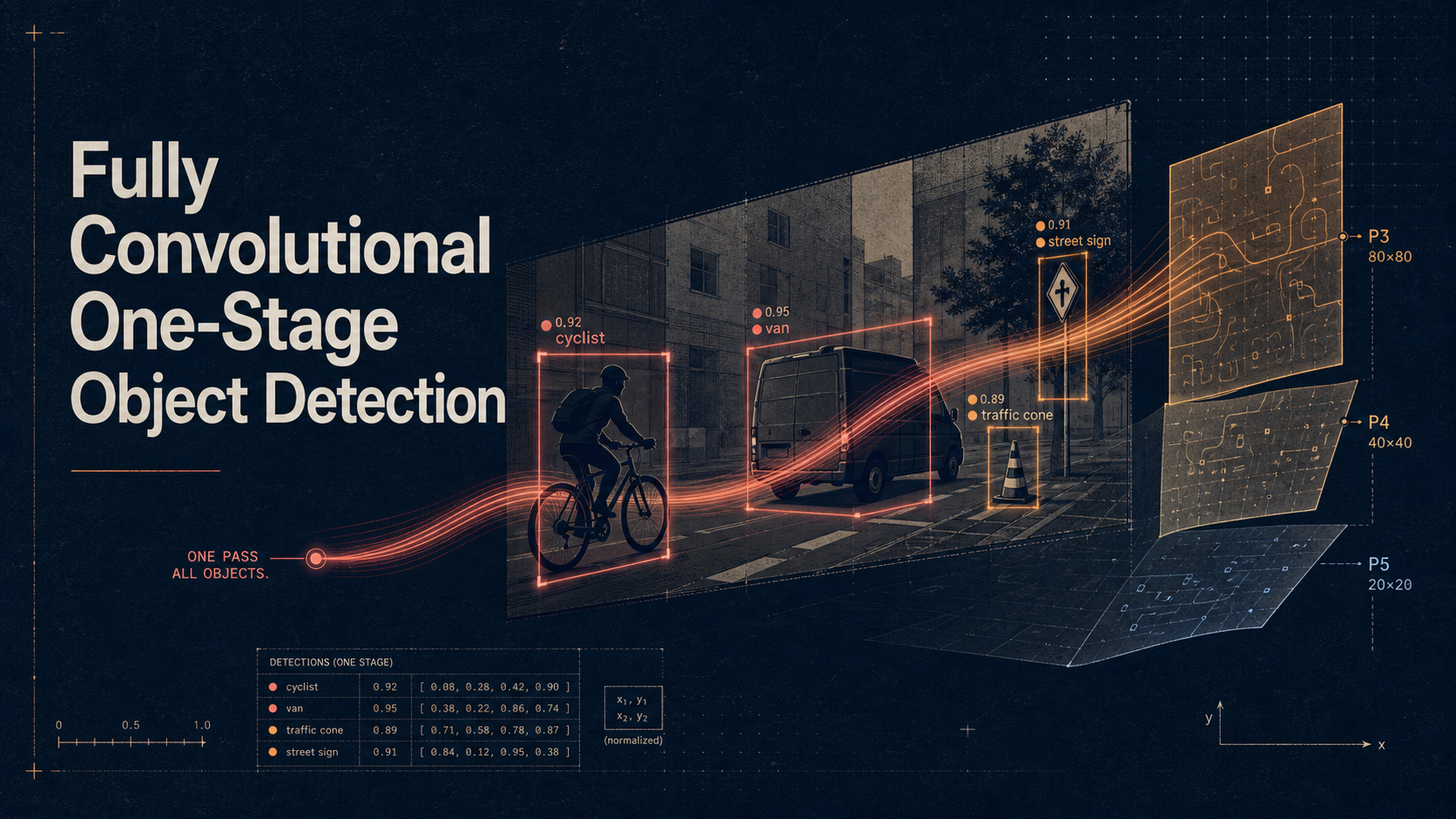
Paper: Zhi Tian, Chunhua Shen, Hao Chen, Tong He — FCOS: Fully Convolutional One-Stage Object Detection, The University of Adelaide, Australia. arXiv: 1904.01355 (this guide is based on v5, 20 Aug 2019) Code released by the authors: tinyurl.com/FCOSv1
This document is a detailed, section-by-section walkthrough of the FCOS paper, written for someone who wants to actually understand why every design choice was made, not just memorize the final numbers. It keeps the original notation, reproduces the key equations, and links the paper’s own figures where they clarify the text. Every ablation table is transcribed in full so you can see exactly which component bought which percentage point of AP.
TL;DR
Object detectors before FCOS almost universally relied on anchor boxes: a dense, hand-designed grid of reference boxes (different scales, different aspect ratios) tiled over the image, which the network then classifies and refines. FCOS asks a simple question: can we detect objects the same way we do semantic segmentation — by making a prediction at every pixel, with no predefined boxes at all?
The answer is yes, and it works better than the anchor-based baselines, not just more simply. FCOS:
- Treats every spatial location on a feature map as a potential training sample (like a pixel in segmentation), and directly regresses the distances from that location to the four sides of the ground-truth box it belongs to.
- Uses a Feature Pyramid Network (FPN) with five prediction levels (P3–P7) to handle objects of different sizes and to resolve the ambiguity of overlapping ground-truth boxes.
- Adds a tiny extra “center-ness” branch — a single convolutional layer — that predicts how close a location is to the center of its target object, so that low-quality, off-center predictions can be down-weighted before non-maximum suppression (NMS).
- Achieves 44.7% AP on COCO
test-devwith a ResNeXt-64x4d-101 backbone, single model, single scale, beating RetinaNet, YOLOv3, SSD, and even the two-stage Faster R-CNN, while removing roughly 9× the number of network outputs anchor boxes would require and every anchor-related hyperparameter. - Doubles as a drop-in, anchor-free replacement for the Region Proposal Network (RPN) inside two-stage detectors like Faster R-CNN, improving average recall there too.
Motivation: What’s Wrong With Anchor Boxes?
Section 1 of the paper opens by pointing out that essentially every mainstream detector of the time — Faster R-CNN, SSD, YOLOv2/v3 — depends on a predefined set of anchor boxes, and that “it has long been believed that the use of anchor boxes is the key to detectors’ success.” The paper pushes back on that belief by cataloguing four concrete drawbacks:
Extreme sensitivity to anchor hyperparameters. Detection performance depends heavily on the sizes, aspect ratios, and number of anchor boxes. The paper cites RetinaNet, where simply varying these hyperparameters swings performance by up to 4% AP on COCO. That is a large amount of accuracy resting on decisions a practitioner has to hand-tune.
Poor generalization to unusual shapes. Because anchor scales and aspect ratios are fixed at design time, detectors struggle with objects that have large shape variation — particularly small objects. Anchors designed for one dataset’s object-size distribution don’t transfer cleanly to a new one; they need to be redesigned.
An enormous, imbalanced set of candidates. To get a high recall rate, anchor-based detectors need to densely tile the image with anchor boxes — the paper notes more than 180K anchor boxes for a single image with shorter side 800 in an FPN-based detector. The overwhelming majority of these are negatives, which worsens the positive/negative imbalance during training.
Expensive matching computation. Assigning anchors to ground truth requires computing Intersection-over-Union (IoU) between every anchor and every ground-truth box, plus additional heuristics (e.g., IoU ≥ 0.5 → positive) that are themselves hyperparameters requiring careful tuning.
At the same time, fully convolutional networks (FCNs) had already produced tremendous per-pixel dense-prediction results in semantic segmentation, depth estimation, keypoint detection, and counting. Object detection was, in the authors’ words, “the only one deviating from the neat fully convolutional per-pixel prediction framework mainly due to the use of anchor boxes.” That observation motivates the paper’s central question:
Can we solve object detection in the neat per-pixel prediction fashion, analogue to FCN for semantic segmentation?
FCOS demonstrates the answer is yes — and that the resulting FCN-based detector is not just simpler but more accurate than its anchor-based counterparts under matched settings.
What FCOS buys you (the paper’s own list of advantages)
- Detection becomes unified with other FCN-solvable dense-prediction tasks, making it easy to reuse ideas across tasks.
- Detection becomes proposal-free and anchor-free, sharply cutting the number of design parameters that need heuristic tuning.
- All anchor-related computation (IoU calculation, anchor–ground-truth matching) disappears entirely, giving faster training/testing and a smaller training memory footprint.
- FCOS achieves state-of-the-art results among one-stage detectors, without any bells and whistles.
- FCOS can be used as the Region Proposal Network inside two-stage detectors, and outperforms anchor-based RPNs there too.
- The framework extends readily to other instance-level vision tasks (e.g., instance segmentation, keypoint detection) with minimal modification.
The FCOS Method
Section 3 of the paper builds the method in three stages: (1) reformulate detection as per-pixel prediction, (2) show how multi-level FPN prediction resolves recall and ambiguity issues, (3) introduce center-ness to suppress low-quality boxes.
Per-pixel prediction: reformulating detection as an FCN task
Let \(F_i \in \mathbb{R}^{H \times W \times C}\) be the feature map at layer \(i\) of a backbone CNN, and let \(s\) be the total stride accumulated up to that layer. The ground-truth boxes for an input image are defined as \(\{B_i\}\), where
\[B_i = (x_0^{(i)}, y_0^{(i)}, x_1^{(i)}, y_1^{(i)}, c^{(i)}) \in \mathbb{R}^4 \times \{1, 2, \dots, C\}\]
Here \((x_0^{(i)}, y_0^{(i)})\) and \((x_1^{(i)}, y_1^{(i)})\) are the left-top and right-bottom corners of the box, \(c^{(i)}\) is the object’s class, and \(C\) is the number of classes (80 for MS-COCO).
For each location \((x, y)\) on feature map \(F_i\), we can map it back to the input image at coordinates \(\left(\lfloor \tfrac{s}{2}\rfloor + xs,\ \lfloor \tfrac{s}{2}\rfloor + ys\right)\), i.e. roughly the center of that location’s receptive field. This is the crucial conceptual shift from anchor-based detectors: anchor-based detectors treat the input-image location as the center of a set of anchor boxes and regress the target box relative to those anchors as references. FCOS instead directly regresses a target box from the location itself — the location is the training sample, exactly as in FCN-based semantic segmentation, rather than being merely the coordinate at which several anchor-box candidates are centered.
Positive / negative assignment. A location \((x,y)\) is a positive sample if it falls inside any ground-truth box, and its class label \(c^*\) is set to that box’s class. Otherwise it is a negative sample with \(c^* = 0\) (background). If a location falls inside more than one ground-truth box, it is called an ambiguous sample — for now, the paper resolves this by simply assigning the ground-truth box with the smallest area as the location’s regression target (multi-level prediction, discussed below, greatly reduces how often this ambiguity actually matters).
Regression targets. For a positive location, the training target is a 4D vector \(\mathbf{t}^* = (l^*, t^*, r^*, b^*)\) — the distances from the location to the left, top, right, and bottom sides of its assigned box. Formally, if location \((x,y)\) is associated with box \(B_i\):
\[l^* = x - x_0^{(i)}, \quad t^* = y - y_0^{(i)}, \quad r^* = x_1^{(i)} - x, \quad b^* = y_1^{(i)} - y \tag{1}\]
This is illustrated directly in the paper’s Figure 1: the left panel shows a positive location inside a baseball player’s bounding box, with arrows depicting exactly the \(l, t, r, b\) distances to be regressed; the right panel shows the ambiguity case, where a single location sits inside two overlapping ground-truth boxes (a tennis player and, presumably, a nearby object) and it isn’t obvious which box’s distances that location should regress.
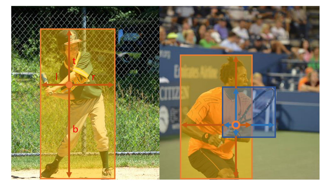
Figure 1 (paper). Left: FCOS predicts a 4D vector \((l, t, r, b)\) at each foreground location, supervised by the ground-truth box it falls inside. Right: when a location falls inside multiple ground-truth boxes, it’s ambiguous which box it should regress against.
Because every location inside a ground-truth box becomes a training sample (not just the ones near the center, and not just the ones with high IoU against a hand-designed anchor), the paper notes that FCOS can “leverage as many foreground samples as possible to train the regressor.” This is a meaningfully different sampling regime from anchor-based detectors, which only treat anchors with sufficiently high IoU against ground truth as positive.
Network outputs. The final layer of the network predicts an 80-D vector \(\mathbf{p}\) of classification probabilities (one binary classifier per class, following RetinaNet’s convention of \(C\) binary classifiers rather than one multi-class softmax) and a 4D vector \(\mathbf{t} = (l, t, r, b)\) of box coordinates. Four convolutional layers are added after the backbone’s feature maps for the classification branch and, separately, for the regression branch (this mirrors RetinaNet’s head design). Because regression targets are always positive, the regression branch’s raw output is passed through \(\exp(x)\) to map any real number onto \((0, \infty)\).
It’s worth pausing on the efficiency claim the authors make explicitly here: FCOS has 9× fewer network output variables than popular anchor-based detectors that use 9 anchor boxes per location. Each location just needs one 4D box plus one class score, instead of nine full sets.
Loss function. The full training loss combines classification and regression terms:
\[L(\{\mathbf{p}_{x,y}\}, \{\mathbf{t}_{x,y}\}) = \frac{1}{N_\text{pos}} \sum_{x,y} L_\text{cls}(\mathbf{p}_{x,y}, c^*_{x,y}) + \frac{\lambda}{N_\text{pos}} \sum_{x,y} \mathbb{1}_{\{c^*_{x,y} > 0\}} L_\text{reg}(\mathbf{t}_{x,y}, \mathbf{t}^*_{x,y}) \tag{2}\]
where \(L_\text{cls}\) is focal loss (as used in RetinaNet) and \(L_\text{reg}\) is the IoU loss (as used in UnitBox). \(N_\text{pos}\) is the number of positive samples, and the balance weight \(\lambda\) is fixed to 1 throughout the paper. The regression loss is masked by the indicator function \(\mathbb{1}_{\{c^*_{x,y}>0\}}\) so it’s only computed at positive locations, and both sums are taken over all locations on feature map \(F_i\) (i.e. over the whole spatial grid, not a sparsely sampled anchor set).
Inference. Inference is described as “straightforward”: forward the image through the network, obtain classification scores \(\mathbf{p}_{x,y}\) and regression predictions \(\mathbf{t}_{x,y}\) at every location, pick locations with \(p_{x,y} > 0.05\) as positive predictions, and invert Equation (1) to reconstruct the predicted bounding box, followed by standard NMS.
Multi-level prediction with FPN
Section 3.2 identifies two potential issues with a plain single-level FCN-based detector, and shows that both are largely solved by borrowing the multi-level prediction idea from Feature Pyramid Networks (FPN).
Issue 1 — low best possible recall (BPR). The best possible recall is the fraction of ground-truth boxes a detector could recall at most, if every positive location were correctly matched — an upper bound on achievable recall. A CNN’s large final stride (e.g. 16×) could, in principle, mean that some objects simply have no feature-map location whose receptive-field center lands inside them, capping recall well below what anchor-based detectors could achieve (anchor-based methods can compensate for large strides by loosening the IoU threshold required for a positive match). The paper empirically shows this fear is largely unfounded for FCOS (see §5.2 below on BPR results): even a single feature level with stride 16 already achieves a BPR of 95.55%, and adding FPN’s multi-level prediction pushes this to 98.40% — very close to the anchor-based RetinaNet’s best achievable 99.23% (as measured in the same Detectron-based training/testing setup).
Issue 2 — ambiguity from overlapping ground-truth boxes. As shown in Figure 1 (right), overlapping ground-truth boxes create locations that could belong to more than one box, and it isn’t intrinsically clear which one a location’s prediction should target. The paper shows this ambiguity is greatly alleviated once objects of very different sizes are assigned to different pyramid levels, because most overlapping happens between objects of considerably different sizes; separating them onto different levels means far fewer locations end up genuinely straddling two ground-truth boxes at the same level.
How multi-level prediction works in FCOS. Following FPN, FCOS detects objects of different sizes on different levels of feature maps, using five levels: \(\{P_3, P_4, P_5, P_6, P_7\}\).
- \(P_3, P_4, P_5\) come from backbone feature maps \(C_3, C_4, C_5\), respectively, followed by a \(1\times1\) convolutional layer with the top-down connections defined in FPN (this is the standard FPN top-down pathway with lateral connections).
- \(P_6\) and \(P_7\) are produced by applying one convolutional layer with stride 2 on top of \(P_5\) and \(P_6\) respectively (i.e., \(P_6\) is derived from \(P_5\), and \(P_7\) from \(P_6\)), extending the pyramid to cover larger objects than the backbone alone reaches.
- As a result, feature levels \(P_3, P_4, P_5, P_6, P_7\) have strides \(8, 16, 32, 64, 128\) respectively.
Unlike anchor-based detectors, which assign anchors of different pre-set sizes to different pyramid levels, FCOS directly limits the range of bounding-box sizes each level is allowed to regress. Concretely: first compute the regression targets \(l^*, t^*, r^*, b^*\) for a location at every level as if that level were responsible; then, if a location satisfies \(\max(l^*, t^*, r^*, b^*) > m_i\) or \(\max(l^*, t^*, r^*, b^*) < m_{i-1}\), it is marked as a negative sample for that level and doesn’t regress a box there at all. Here \(m_i\) is the maximum distance that feature level \(i\) is allowed to regress. In this paper, \(m_2, m_3, m_4, m_5, m_6, m_7\) are set to \(0, 64, 128, 256, 512, \infty\) respectively (so, e.g., \(P_3\) handles objects whose max side-distance is in \([0, 64]\), \(P_4\) handles \([64, 128]\), and so on up to \(P_7\) handling anything larger than 512).
If, even after this level-based split, a location is still assigned to more than one ground-truth box at the same level (i.e., genuine same-level overlap), FCOS falls back to the same rule as before — choose the ground-truth box with minimal area as the regression target. The paper’s empirical measurements (Table 2, below) show this residual ambiguity is small once FPN-based level splitting is applied.
Head sharing, but with a per-level scalar. Following FPN and RetinaNet, FCOS shares detection heads across the different feature levels, which both keeps the detector parameter-efficient and, empirically, improves detection performance versus using separate heads per level. However, different feature levels are responsible for regressing different size ranges (e.g. \([0,64]\) for \(P_3\) vs \([64,128]\) for \(P_4\)), so it would be unreasonable for every level to use an identical output transform. Instead of the standard \(\exp(x)\) used to map the raw regression output onto \((0,\infty)\), FCOS uses \(\exp(s_i x)\) with a trainable scalar \(s_i\) specific to level \(P_i\), which automatically adjusts the exponential’s base per level and slightly improves detection performance.
The architecture end to end
Putting the backbone, FPN, and heads together gives the full FCOS architecture shown in the paper’s Figure 2. Reading left to right: an input image (example dimensions \(800\times1024\)) is passed through the backbone to produce feature maps \(C_3, C_4, C_5\) at strides \(8, 16, 32\); a top-down FPN pathway with \(1\times1\) lateral connections turns these into \(P_3, P_4, P_5\), which are then extended with two extra stride-2 convolutions to produce \(P_6\) (stride 64) and \(P_7\) (stride 128); each of the five pyramid levels is fed through a shared detection head that branches into three sibling outputs — classification (\(H\times W\times C\)), center-ness (\(H\times W\times 1\)), and regression (\(H\times W\times 4\)) — each produced by its own stack of 4 convolutional layers before the final \(1\times1\) projection.
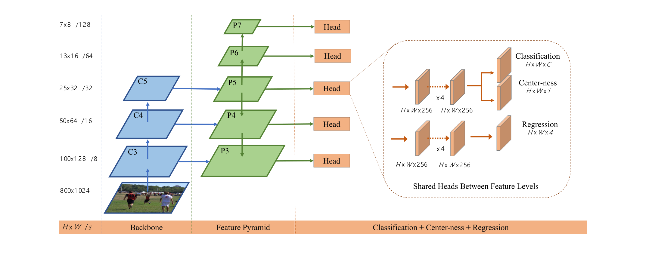
Figure 2 (paper). C3, C4, C5 are backbone feature maps; P3–P7 are the FPN levels used for final prediction. H×W is the feature-map resolution at that level, and ‘/s’ is the downsampling ratio relative to the 800×1024 input image (s = 8, 16, 32, 64, 128). The shared head on the right produces classification, center-ness, and regression outputs per level.
Note in the original figure that the center-ness branch is drawn in parallel with the classification branch. The paper flags in a footnote that after the initial submission, it was shown that AP can be improved slightly if center-ness is instead placed in parallel with the regression branch — but unless otherwise specified, the paper still reports results using the classification-branch configuration shown in Figure 2.
For readability, here is the same architecture redrawn as a Mermaid flowchart, with the size/stride annotations from the figure preserved:
flowchart LR
    subgraph INPUT["Input"]
        IMG["Input image<br/>800 × 1024"]
    end

    subgraph BACKBONE["Backbone"]
        C3["C3<br/>100×128 · stride 8"]
        C4["C4<br/>50×64 · stride 16"]
        C5["C5<br/>25×32 · stride 32"]
        IMG --> C3 --> C4 --> C5
    end

    subgraph FPN["Feature Pyramid"]
        P3["P3<br/>100×128 · stride 8"]
        P4["P4<br/>50×64 · stride 16"]
        P5["P5<br/>25×32 · stride 32"]
        P6["P6<br/>13×16 · stride 64"]
        P7["P7<br/>7×8 · stride 128"]
        C3 -- "1×1 conv + lateral" --> P3
        C4 -- "1×1 conv + lateral" --> P4
        C5 -- "1×1 conv + top-down" --> P5
        P5 -- "stride-2 conv" --> P6
        P6 -- "stride-2 conv" --> P7
    end

    subgraph HEAD["Shared Head (per level)"]
        direction TB
        CLS_STACK["4× conv, 256 ch<br/>(classification tower)"]
        REG_STACK["4× conv, 256 ch<br/>(regression tower)"]
        CLS["Classification<br/>H×W×C"]
        CTR["Center-ness<br/>H×W×1"]
        REG["Regression<br/>H×W×4<br/>(l, t, r, b)"]
        CLS_STACK --> CLS
        CLS_STACK --> CTR
        REG_STACK --> REG
    end

    P3 --> HEAD
    P4 --> HEAD
    P5 --> HEAD
    P6 --> HEAD
    P7 --> HEAD

    HEAD --> OUT["Per-location predictions<br/>at every level → NMS"]
A second way to see the method — as the data flow of a single training sample rather than the network’s module graph — makes the anchor-free logic explicit:
flowchart TD
    A["Location (x, y) on feature map P_i, stride s"] --> B{"Does (x, y) map inside<br/>any ground-truth box?"}
    B -- "No" --> N["Negative sample<br/>c* = 0 (background)"]
    B -- "Yes" --> C{"Inside more than<br/>one GT box at this level?"}
    C -- "No" --> D["Positive sample<br/>c* = class of that box"]
    C -- "Yes, ambiguous" --> E["Pick GT box with<br/>minimal area"]
    E --> D
    D --> F["Compute regression target<br/>t* = (l*, t*, r*, b*)<br/>distances to the 4 sides"]
    F --> G{"max(l*,t*,r*,b*) within<br/>this level's range [m_i-1, m_i]?"}
    G -- "No" --> N
    G -- "Yes" --> H["Train classification + regression + center-ness<br/>at this location"]
Center-ness for FCOS
Even after multi-level FPN prediction closes most of the recall/ambiguity gap, Section 3.3 notes there is still a performance gap between FCOS and anchor-based detectors. The diagnosed cause: FCN-based FCOS produces a lot of low-quality detected bounding boxes from locations that are far from the center of an object — a location near the edge of a person’s bounding box, for instance, can still technically be “inside” the box and thus a valid positive sample, but its regression prediction tends to be much noisier than a location near the object’s center.
The fix is a single extra convolutional layer, run in parallel with the classification branch, that predicts a scalar “center-ness” score for each location, without introducing any new hyperparameters. Given the regression targets \(l^*, t^*, r^*, b^*\) for a location, the center-ness target is defined as:
\[\text{centerness}^* = \sqrt{\frac{\min(l^*, r^*)}{\max(l^*, r^*)} \times \frac{\min(t^*, b^*)}{\max(t^*, b^*)}} \tag{3}\]
This quantity ranges from 0 (at the edge of the box) to 1 (exactly at the center), and the square root is used specifically to slow down the decay of center-ness as a location moves away from the center — i.e., without the square root the score would fall off more sharply, and the authors found slowing that decay works better. It is trained with binary cross-entropy (BCE) loss, added directly onto the loss in Equation (2).
The paper’s Figure 3 visualizes exactly this quantity for a photo of a child: the heatmap overlay shows center-ness decaying smoothly from 1 (red, at the object’s center) outward to 0 as you approach any of the four sides (\(l^*, t^*, r^*, b^*\) are drawn explicitly on the image).
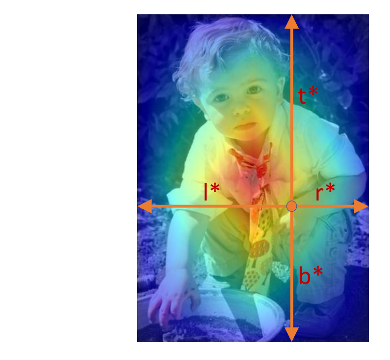
Figure 3 (paper). Red, blue, and intermediate colors denote center-ness values of 1, 0, and values in between. Center-ness is computed by Equation (3) and decays from 1 to 0 as a location moves away from the object’s center.
How it’s used at inference. The predicted center-ness score is multiplied with the classification score to produce the final ranking score used for NMS. This means a location that is confidently classified but sits far from the object’s center gets its score pulled down before NMS ever runs, so these low-quality boxes are much more likely to be filtered out — improving detection performance “remarkably,” in the paper’s words.
Visual confirmation (Appendix, Section 8 / Figure 7). The paper backs this mechanism with a striking scatter plot. Treat each detected bounding box as a 2D point \((x, y)\) where \(x\) is the box’s confidence score and \(y\) is its true IoU with its corresponding ground-truth box. Before applying center-ness (Figure 7, left), there is a large mass of points with high confidence but low IoU — exactly the low-quality boxes that are dangerous because NMS can’t tell they’re bad from the score alone. After multiplying classification score by center-ness (Figure 7, right), that same population is pushed to the left (lower score), separating high-confidence points more cleanly along the high-IoU diagonal.
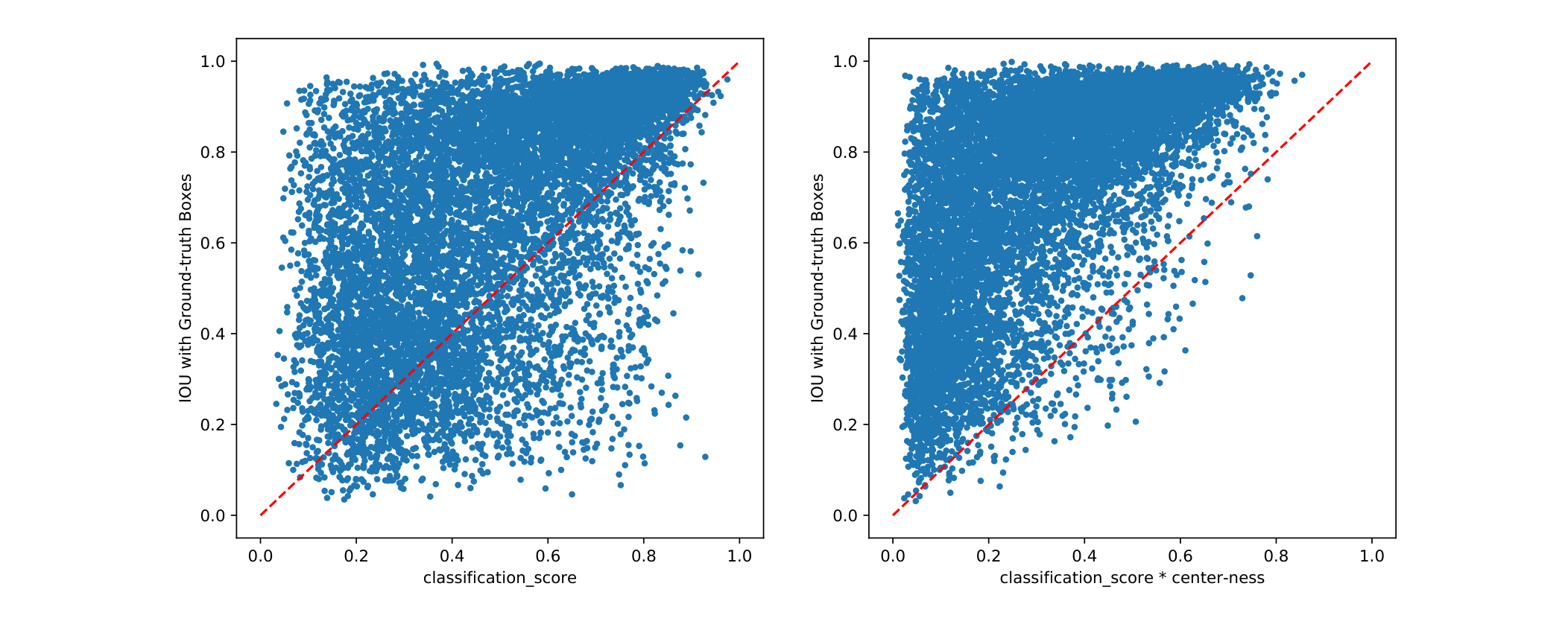
Figure 7 (paper). Each point is a detected box. Left: without center-ness, many boxes have high classification score but low IoU with ground truth (the dangerous, hard-to-filter low-quality boxes). Right: after multiplying scores by predicted center-ness, those same low-quality boxes are pushed toward lower scores.
An alternative the paper explicitly rules out (mostly). One could compute an analogous “center-ness” quantity directly from the predicted regression vector instead of learning a separate branch — this needs no extra parameters at all. Later works (cited as [12], [33], and post-submission work [1]) showed this can work if combined with only sampling the central portion of the ground-truth box as positive (“center sampling”). The ablation table in Section 4.1.2 (Table 4, reproduced below) shows that on its own, computing center-ness purely from the regression vector does not improve performance — the separate, learned center-ness branch is necessary.
Experiments
All experiments use the large-scale COCO benchmark. Following common practice, the paper trains on the trainval35k split (115K images), validates ablations on minival (5K images), and reports final test numbers on test-dev (20K images) via the evaluation server.
Training and inference details
- Backbone: ResNet-50 unless otherwise specified, using the same hyperparameters as RetinaNet.
- Optimizer: SGD for 90K iterations, initial learning rate 0.01, mini-batch size 16; learning rate reduced ×10 at iterations 60K and 80K.
- Regularization: weight decay 0.0001, momentum 0.9.
- Initialization: backbone pretrained on ImageNet; newly added layers initialized as in RetinaNet.
- Image sizes: shorter side resized to 800, longer side capped at 1333 (both training and testing), unless otherwise specified.
- Inference: forward pass → predicted boxes with class scores → same post-processing hyperparameters as RetinaNet (including the same NMS settings) → final detections.
Best possible recall: is FCOS’s large stride actually a problem?
This directly answers Concern #1 raised in §4.2 above. Table 1 compares the BPR of anchor-based RetinaNet under different matching rules against FCN-based FCOS:
| Method | w/ FPN | Low-quality matches | BPR (%) |
|---|---|---|---|
| RetinaNet | ✓ | None | 86.82 |
| RetinaNet | ✓ | ≥ 0.4 | 90.92 |
| RetinaNet | ✓ | All | 99.23 |
| FCOS | – | 95.55 | |
| FCOS | ✓ | – | 98.40 |
Table 1 (paper). BPR for anchor-based RetinaNet under a variety of matching rules, vs. FCN-based FCOS. FCOS’s recall is very close to the best anchor-based number, and much higher than RetinaNet’s official Detectron implementation (which only uses low-quality matches with IoU ≥ 0.4).
Reading this table carefully: with no FPN — i.e., a single feature level at stride 16 (\(P_4\)) — FCOS already reaches a BPR of 95.55%, comfortably above RetinaNet’s official implementation number of 90.92% (which only uses IoU ≥ 0.4 matches). Adding FPN pushes FCOS to 98.40%, within about 1 percentage point of the theoretical maximum an anchor-based detector could reach (99.23%, achieved only by allowing all low-quality matches, which real detectors don’t actually use because it would hurt precision). The paper’s conclusion: the low-BPR concern about FCN-based detection is not actually a problem in practice, and the small residual gap (under 1%) doesn’t measurably hurt final AR/AP, as confirmed later in Table 3.
Ambiguous samples: how much does overlap actually hurt?
This answers Concern #2. Table 2 measures the fraction of positive samples that are “ambiguous” (fall inside more than one ground-truth box):
| w/ FPN | Amb. samples (%) | Amb. samples (diff.) (%) |
|---|---|---|
| 23.16 | 17.84 | |
| ✓ | 7.14 | 3.75 |
Table 2 (paper). “Amb. samples” = ratio of ambiguous samples to all positive samples. “Amb. samples (diff.)” is similar but excludes ambiguity between objects of the same category, since which of two same-class overlapping boxes a location regresses doesn’t actually matter for the final prediction.
Without FPN, 23.16% of positive samples are technically ambiguous. With FPN’s per-level size-range splitting, this drops to 7.14% — because most overlapping objects differ considerably in size and therefore land on different pyramid levels automatically. If you additionally only count ambiguity between objects of different classes (since misassigning between two same-class overlapping boxes doesn’t change the predicted class, only which specific instance’s coordinates get regressed — usually harmless), the ratio falls further, to 3.75%. The paper additionally measured, at inference time, that only 2.3% of detected boxes come from ambiguous locations at all, and only 1.5% once same-class overlaps are excluded — and even those don’t necessarily represent an error, since ambiguous locations are always assigned the box with minimal area, so they primarily risk missing a larger overlapping object rather than mispredicting entirely (a larger object typically also has other, unambiguous locations available to predict it).
Ablation: With or without center-ness
Table 4 isolates the contribution of the center-ness branch, on minival with ResNet-50-FPN:
| AP | AP₅₀ | AP₇₅ | AP_S | AP_M | AP_L | |
|---|---|---|---|---|---|---|
| None | 33.5 | 52.6 | 35.1 | 20.8 | 38.5 | 42.6 |
| center-ness† | 33.5 | 52.4 | 35.1 | 20.8 | 37.8 | 42.8 |
| center-ness | 37.1 | 55.9 | 39.8 | 21.3 | 41.0 | 47.8 |
Table 4 (paper). “None” = no center-ness at all. “center-ness†” = center-ness computed from the predicted regression vector (no extra branch). “center-ness” = the proposed learned center-ness branch.
The result is unambiguous: computing center-ness for free from the regression vector (center-ness†) gives essentially no improvement over having no center-ness at all (33.5 → 33.5 AP). The dedicated, jointly-trained center-ness branch, however, is worth +3.6 AP (33.5 → 37.1), with the largest single-column gains on AP₅₀, AP₇₅, and AP_L. This is the empirical justification for why the extra branch — cheap as it is (one conv layer) — earns its place in the architecture.
FCOS vs. Anchor-based Detectors, Head-to-Head (Table 3)
Table 3 is the paper’s central ablation, walking from a vanilla single-level RetinaNet-style setup all the way to the fully improved FCOS, isolating each contribution along the way:
| Method | \(C_5\)/\(P_5\) | w/ GN | nms thr. | AP | AP₅₀ | AP₇₅ | AP_S | AP_M | AP_L | AR₁ | AR₁₀ | AR₁₀₀ |
|---|---|---|---|---|---|---|---|---|---|---|---|---|
| RetinaNet | \(C_5\) | .50 | 35.9 | 56.0 | 38.2 | 20.0 | 39.8 | 47.4 | 31.0 | 49.2 | 52.5 | |
| FCOS | \(C_5\) | .50 | 36.3 | 54.9 | 38.7 | 20.5 | 39.8 | 47.8 | 31.5 | 50.6 | 53.3 | |
| FCOS | \(P_5\) | .50 | 36.4 | 54.9 | 39.3 | 19.7 | 39.7 | 53.4 | 31.4 | 50.6 | 53.4 | |
| FCOS | \(P_5\) | .60 | 36.5 | 59.2 | 39.2 | 19.8 | 40.0 | 48.9 | 31.3 | 51.2 | 54.5 | |
| FCOS | \(P_5\) | ✓ | .60 | 37.1 | 55.9 | 39.8 | 21.3 | 40.0 | 48.9 | 31.4 | 51.4 | 54.9 |
| + ctr. on reg. | \(P_5\) | ✓ | .60 | 37.4 | 56.1 | 40.3 | 21.8 | 41.2 | 48.8 | 31.5 | 51.7 | 55.2 |
| + ctr. sampling [1] | \(P_5\) | ✓ | .60 | 38.1 | 56.7 | 41.4 | 22.6 | 41.6 | 56.3 | 32.1 | 52.8 | 56.3 |
| + GIoU [1] | \(P_5\) | ✓ | .60 | 38.3 | 57.1 | 41.0 | 21.9 | 42.4 | 49.5 | 32.0 | 52.9 | 56.5 |
| + Normalization | \(P_5\) | ✓ | .60 | 38.6 | 57.4 | 42.4 | 22.3 | 42.5 | 49.8 | 32.3 | 53.4 | 57.1 |
(Table 3, reproduced with all columns — some numbers, e.g. FCOS \(P_5\) AP_L jumps, are transcribed as printed in the source.) “ctr. on reg.”: moves the center-ness branch to run parallel with the regression branch instead of classification. “ctr. sampling”: only samples the central portion of a ground-truth box’s area as positive. “GIoU”: penalizes the union area over the circumscribed rectangle’s area, added to the IoU loss. “Normalization”: normalizes the regression targets in Equation (1) using each FPN level’s stride.
Two things stand out. First, with exactly matched training and testing settings, a bare-bones FCOS already edges out RetinaNet (36.3 vs. 35.9 AP) — the anchor-free reformulation isn’t just simpler, it’s already at least as good with zero extra tricks. Second, a sequence of “almost cost-free improvements” — discovered after the original submission — stack up to a much larger gain: using \(P_5\) instead of \(C_5\) to derive \(P_6\)/\(P_7\), adding Group Normalization (GN) in the head, raising the NMS threshold to 0.6, moving center-ness to the regression branch, adding center sampling, GIoU loss, and normalizing regression targets by stride together lift AP from 36.3 all the way to 38.6 — a total improvement of +2.3 AP over the already-competitive baseline, achieved without adding meaningful complexity.
Comparison with State-of-the-art Detectors (Table 5)
Table 5 is the paper’s headline results table on test-dev, single-model and single-scale:
| Method | Backbone | AP | AP₅₀ | AP₇₅ | AP_S | AP_M | AP_L |
|---|---|---|---|---|---|---|---|
| Two-stage: | |||||||
| Faster R-CNN w/ FPN | ResNet-101-FPN | 36.2 | 59.1 | 39.0 | 18.2 | 39.0 | 48.2 |
| Faster R-CNN by G-RMI | Inception-ResNet-v2 | 34.7 | 55.5 | 36.7 | 13.5 | 38.1 | 52.0 |
| Faster R-CNN w/ TDM | Inception-ResNet-v2-TDM | 36.8 | 57.7 | 39.2 | 16.2 | 39.8 | 52.1 |
| One-stage: | |||||||
| YOLOv2 | DarkNet-19 | 21.6 | 44.0 | 19.2 | 5.0 | 22.4 | 35.5 |
| SSD513 | ResNet-101-SSD | 31.2 | 50.4 | 33.3 | 10.2 | 34.5 | 49.8 |
| DSSD513 | ResNet-101-DSSD | 33.2 | 53.3 | 35.2 | 13.0 | 35.4 | 51.1 |
| RetinaNet | ResNet-101-FPN | 39.1 | 59.1 | 42.3 | 21.8 | 42.7 | 50.2 |
| CornerNet | Hourglass-104 | 40.5 | 56.5 | 43.1 | 19.4 | 42.7 | 53.9 |
| FSAF | ResNeXt-64x4d-101-FPN | 42.9 | 63.8 | 46.3 | 26.6 | 46.2 | 52.7 |
| FCOS | ResNet-101-FPN | 41.5 | 60.7 | 45.0 | 24.4 | 44.8 | 51.6 |
| FCOS | HRNet-W32-5l | 42.0 | 60.4 | 45.3 | 25.4 | 45.0 | 51.0 |
| FCOS | ResNeXt-32x8d-101-FPN | 42.7 | 62.4 | 46.1 | 26.0 | 45.6 | 52.6 |
| FCOS w/ improvements | ResNeXt-64x4d-101-FPN | 44.7 | 64.1 | 48.4 | 27.6 | 47.5 | 55.6 |
Table 5 (paper). Single-model, single-scale results. FCOS outperforms anchor-based RetinaNet by 2.4 AP with the same backbone, and outperforms the anchor-free CornerNet with much less design complexity.
With the same ResNet-101-FPN backbone, FCOS beats RetinaNet by 2.4 AP (41.5 vs. 39.1). It’s also the first time, per the authors, that an anchor-free detector — without any bells and whistles — outperforms anchor-based detectors by this large a margin. With the improvements from §5.5 folded in and a ResNeXt-64x4d-101-FPN backbone, FCOS reaches 44.7% AP, surpassing every detector listed, including the two-stage Faster R-CNN variants and the anchor-free CornerNet (which additionally requires learned corner-grouping machinery FCOS doesn’t need at all).
Extension: FCOS as a Region Proposal Network
Section 5 tests whether FCOS’s anchor-free machinery also works as a drop-in replacement for the anchor-based RPN inside two-stage Faster R-CNN. The only changes: anchor boxes in the RPN are replaced by FCOS-style FPN prediction, and Group Normalization is added into the FPN head layers for training stability; everything else matches the official Faster R-CNN + FPN RPN code.
| Method | # samples | AR¹⁰⁰ | AR¹ᴷ |
|---|---|---|---|
| RPN w/ FPN & GN (ReImpl.) | ~200K | 44.7 | 56.9 |
| FCOS w/o center-ness | ~66K | 48.0 | 59.3 |
| FCOS w/ GN | ~66K | 52.8 | 60.3 |
Table 6 (paper). ResNet-50 backbone. FCOS improves AR¹⁰⁰ and AR¹ᴷ by 8.1% and 3.4% respectively over RPN with FPN.
Even without center-ness, FCOS’s RPN variant improves both AR¹⁰⁰ and AR¹ᴷ significantly over the anchor-based RPN — despite using roughly 3× fewer samples (~66K vs. ~200K). Adding the center-ness branch pushes AR¹⁰⁰ to 52.8% (an 18% relative improvement) and AR¹ᴷ to 60.3% (a 3.4 percentage-point absolute improvement) over the anchor-based RPN baseline.
Appendix Material
Class-agnostic precision-recall curves
The appendix (Section 7) reports class-agnostic PR curves — i.e., detection quality ignoring which class was predicted, purely measuring localization — at three IoU thresholds: 0.50, 0.75, and 0.90.
| Method | AP | AP₅₀ | AP₇₅ | AP₉₀ |
|---|---|---|---|---|
| Original RetinaNet | 39.5 | 63.6 | 41.8 | 10.6 |
| RetinaNet w/ GN | 40.0 | 64.5 | 42.2 | 10.4 |
| FCOS | 40.5 | 64.7 | 42.6 | 13.1 |
| (FCOS − RetinaNet w/ GN) | +0.5 | +0.2 | +0.4 | +2.7 |
Table 7 (paper). Class-agnostic detection performance. FCOS’s improvement over RetinaNet grows as the IoU threshold gets stricter.
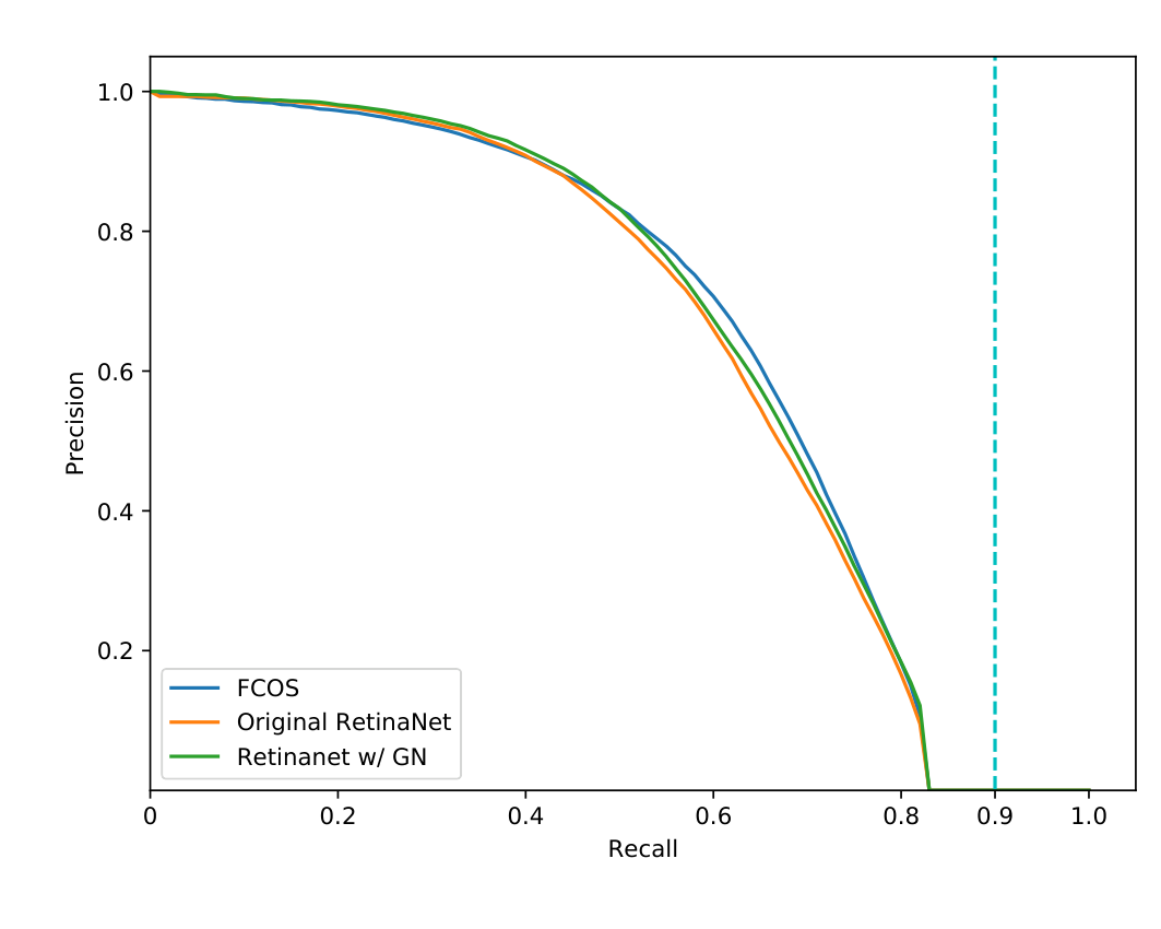
Figure 4 (paper). Class-agnostic precision-recall curves at IoU = 0.50.
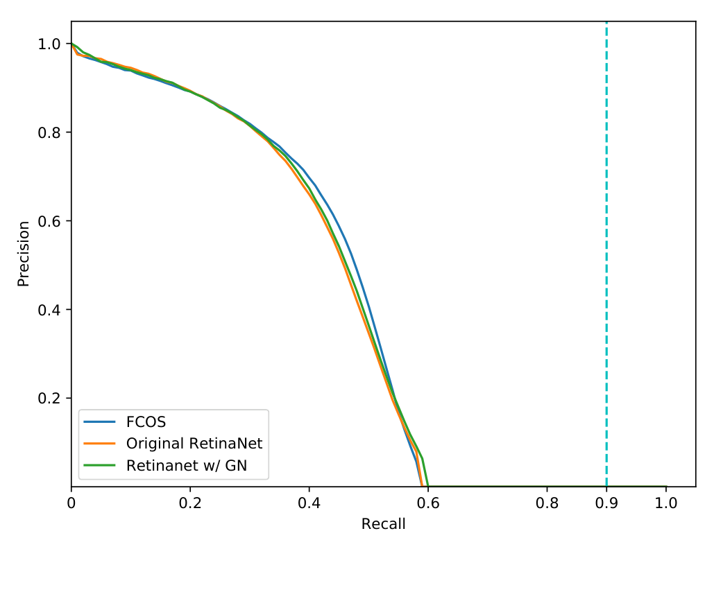
Figure 5 (paper). Class-agnostic precision-recall curves at IoU = 0.75.
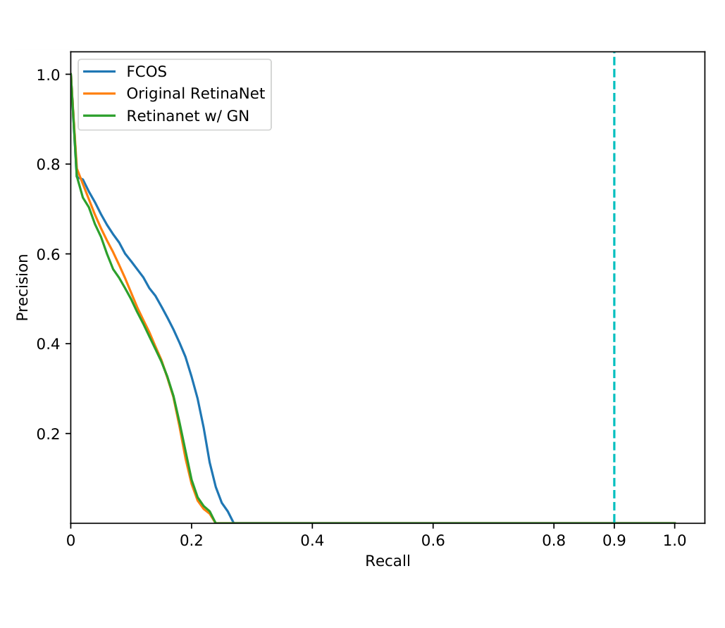
Figure 6 (paper). Class-agnostic precision-recall curves at IoU = 0.90.
The key pattern across all three curves: FCOS’s advantage over RetinaNet grows as the IoU threshold gets stricter (+0.2 at IoU 0.50, growing to +2.7 at IoU 0.90). The paper interprets this as evidence that FCOS produces a better bounding-box regressor — more accurate localization, not just more confident classification — which it attributes to FCOS being able to leverage many more foreground training samples (every location inside a box, not just anchors with sufficient IoU) to train the regressor. It’s also worth noting, as the paper does, that the best recall achievable by any of these detectors in these curves is well under 90% — meaning the small BPR gap between FCOS (98.40%) and the anchor-based upper bound (99.23%) discussed in §5.2 is far too small to be the bottleneck on final detection performance.
Qualitative results
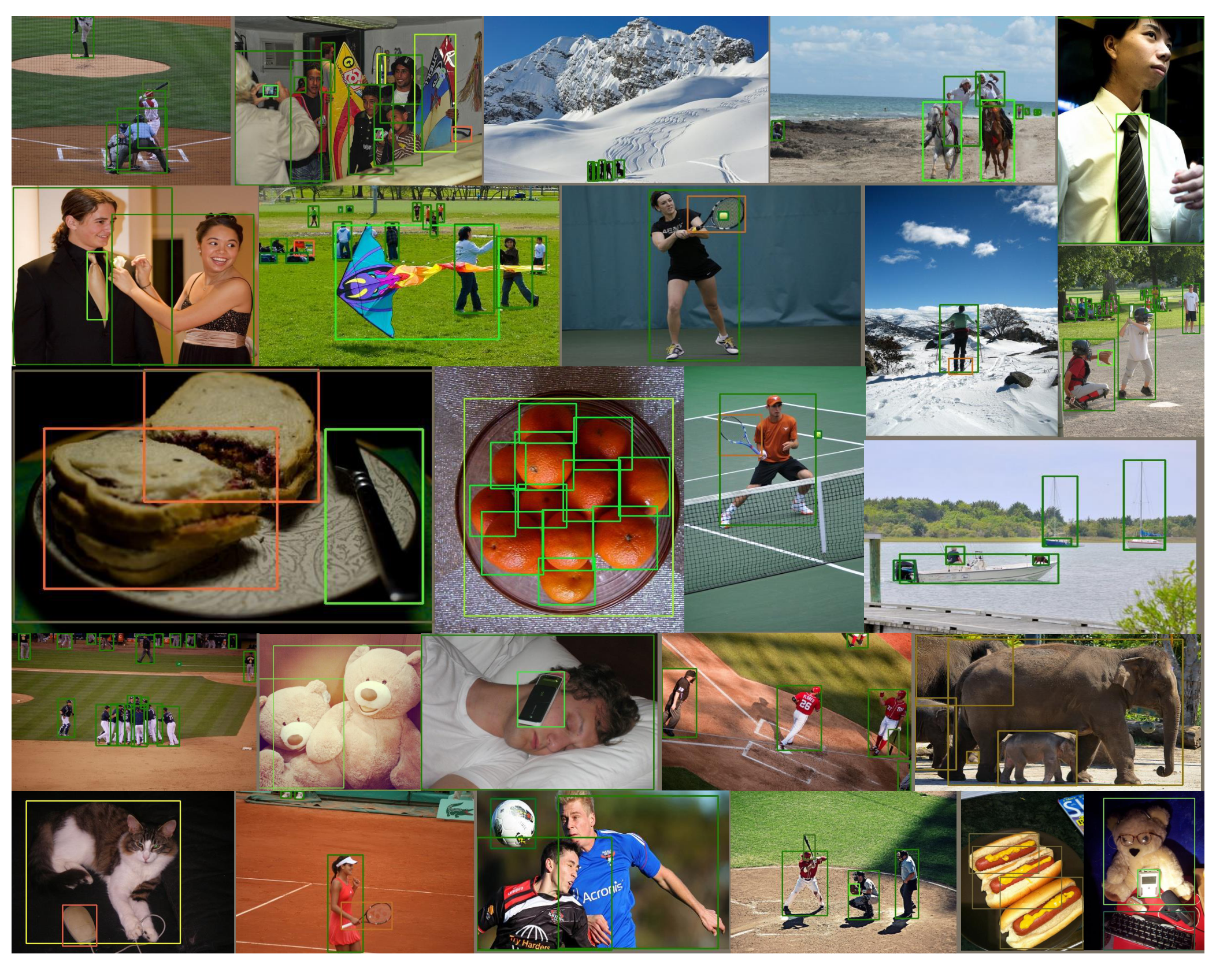
Figure 8 (paper). Detection results on the minival split with a ResNet-50 backbone. FCOS handles crowded scenes, occlusion, highly overlapped instances, extremely small objects, and very large objects.
The grid in Figure 8 is a useful sanity check on everything argued above in prose: crowded scenes (the group photo, the baseball infield), heavily occluded and overlapping instances (the pile of oranges, the two soccer players colliding), and objects at extreme scale — from a person barely visible on a distant mountainside to an elephant filling most of the frame — are all detected with reasonable bounding boxes, which is exactly the “wide range of object candidates with large shape variations” case that Section 2 of this guide identified as a weak point for fixed-anchor detectors.
Further discussion (Section 10 of the paper)
A few clarifying points the authors add in a final discussion section:
- Center-ness vs. IoUNet. Center-ness shares a similar goal with IoUNet (Jiang et al.), which trains a separate network to predict IoU between a predicted box and its ground truth. Center-ness is much simpler: it’s a single layer trained jointly with the rest of the detector, and — unlike IoUNet — it does not take the predicted bounding box as input at all; it only looks at the location’s intrinsic geometric relationship to the object.
- On the BPR discussion. The authors clarify that Table 1’s BPR numbers shouldn’t be over-interpreted as “recall by specific IoU” — its main purpose is just to show FCOS’s recall ceiling is close to the anchor-based ceiling (98.40% vs 99.23%). They explicitly state there is no evidence FCOS’s regression targets are harder to learn because they’re more spread out; in fact FCOS produces more accurate boxes, per Table 7.
- Ambiguity at inference, restated. Because the minimal-area rule is used consistently, a mistake in ambiguous locations (Table 2) can only occur when two overlapping objects belong to different classes and a location predicts the wrong one’s class alongside the other’s coordinates — this is why the paper separately reports the “different-class-only” ambiguity ratio.
- Additional ablation study (Table 8,
minival):
| Method | \(C_5\)/\(P_5\) | GN | Scalar | IoU | AP |
|---|---|---|---|---|---|
| RetinaNet (#A=1) | \(C_5\) | 32.5 | |||
| RetinaNet (#A=9) | \(C_5\) | 35.7 | |||
| FCOS (pure) | \(C_5\) | 35.7 | |||
| FCOS | \(P_5\) | 35.8 | |||
| FCOS | \(P_5\) | ✓ | 36.3 | ||
| FCOS | \(P_5\) | ✓ | ✓ | 36.4 | |
| FCOS | \(P_5\) | ✓ | ✓ | ✓ | 36.6 |
Table 8 (paper). “#A” is the number of anchor boxes per location in RetinaNet. “IoU” here denotes IoU loss for regression. “Scalar” denotes whether the trainable per-level scalar \(s_i\) is used in exp(\(s_i x\)). All experiments use matched settings.
This table makes an important simplicity point on its own: a “pure” vanilla FCOS (35.7 AP) performs on par with RetinaNet using 9 anchors per location (35.7 AP) — i.e., FCOS matches full anchor-based RetinaNet with ~9× fewer network outputs and zero anchor hyperparameters — and clearly beats RetinaNet restricted to a single anchor per location (32.5 AP), which is the fairer point of comparison for an inherently single-box-per-location detector like FCOS.
- Center-ness can’t be added directly to multi-anchor RetinaNet, because a location on the feature map has only one center-ness score, whereas RetinaNet’s multiple anchor boxes at the same location would each need their own “soft” positive/negative threshold — center-ness and IoU-based anchor thresholds aren’t directly interchangeable in that setting.
- Positive samples overlap with RetinaNet, clarified. Center-ness only comes into play at test time for score re-ranking. During training, all locations within ground-truth boxes are marked positive regardless of center-ness, which is precisely why FCOS gets to use more foreground locations to train its regressor than an IoU-thresholded anchor matching scheme would.
Conclusion (Section 6 of the paper, expanded)
FCOS is proposed as an anchor-free, proposal-free one-stage object detector. It compares favorably against popular anchor-based one-stage detectors (RetinaNet, YOLO, SSD) while removing essentially all anchor-related computation and hyperparameters. Conceptually, FCOS solves detection in a per-pixel prediction fashion, putting it in the same family as other dense-prediction FCN tasks like semantic segmentation, and it achieves state-of-the-art performance among one-stage detectors as a result. The paper also demonstrates FCOS working as an RPN inside a two-stage detector, again outperforming the anchor-based counterpart. Given its effectiveness, efficiency, and — above all — its simplicity, the authors position FCOS as a strong, general-purpose alternative to anchor-based detection, and suggest it could serve as a baseline for other instance-level recognition tasks going forward.
Why this paper mattered
Stepping back from the paper’s own framing: FCOS was one of the influential papers (alongside CornerNet and later works like CenterNet, ATSS, and FCOS’s own descendants) that pushed the object-detection field away from anchor-based design as a default assumption. The center-ness idea in particular — a cheap, jointly-trained quality-estimation signal used purely to re-rank detections before NMS — became a recurring pattern in later anchor-free and even some anchor-based detectors. Practically, its adoption in production systems (e.g., as the detection head in several instance-segmentation and video-detection pipelines that followed) was helped enormously by exactly the properties the paper emphasizes: fewer hyperparameters to tune, fewer outputs to compute, and a training/inference pipeline that maps cleanly onto standard FCN dense-prediction infrastructure.
Key Equations, Collected
For quick reference, the paper’s three core equations:
(1) Regression targets for a positive location \((x,y)\) assigned to ground-truth box \(B_i = (x_0^{(i)}, y_0^{(i)}, x_1^{(i)}, y_1^{(i)})\):
\[l^* = x - x_0^{(i)}, \qquad t^* = y - y_0^{(i)}, \qquad r^* = x_1^{(i)} - x, \qquad b^* = y_1^{(i)} - y\]
(2) Training loss, combining focal loss for classification and IoU loss for regression, normalized by the number of positive samples \(N_\text{pos}\):
\[L = \frac{1}{N_\text{pos}} \sum_{x,y} L_\text{cls}(\mathbf{p}_{x,y}, c^*_{x,y}) + \frac{\lambda}{N_\text{pos}} \sum_{x,y} \mathbb{1}_{\{c^*_{x,y} > 0\}} L_\text{reg}(\mathbf{t}_{x,y}, \mathbf{t}^*_{x,y})\]
(3) Center-ness target, ranging over \([0, 1]\):
\[\text{centerness}^* = \sqrt{\frac{\min(l^*, r^*)}{\max(l^*, r^*)} \times \frac{\min(t^*, b^*)}{\max(t^*, b^*)}}\]
References (as cited in the paper)
The reference numbers below match the in-text citation numbers used throughout this guide and the original paper.
https://github.com/yqyao/FCOS_PLUS, 2019.- Boominathan, Kruthiventi, Babu. CrowdNet: A deep convolutional network for dense crowd counting. ACM Multimedia, 2016.
- Chen, Shen, Wei, Liu, Yang. Adversarial PoseNet: A structure-aware convolutional network for human pose estimation. ICCV, 2017.
- Deng, Dong, Socher, Li, Li, Fei-Fei. ImageNet: A large-scale hierarchical image database. CVPR, 2009.
- Fu, Liu, Ranga, Tyagi, Berg. DSSD: Deconvolutional single shot detector. arXiv:1701.06659, 2017.
- Girshick. Fast R-CNN. ICCV, 2015.
- Girshick, Radosavovic, Gkioxari, Dollár, He. Detectron.
github.com/facebookresearch/detectron, 2018. - He, Zhang, Ren, Sun. Deep residual learning for image recognition. CVPR, 2016.
- He, Shen, Tian, Gong, Sun, Yan. Knowledge adaptation for efficient semantic segmentation. CVPR, June 2019.
- He, Tian, Huang, Shen, Qiao, Sun. An end-to-end textspotter with explicit alignment and attention. CVPR, 2018.
- Huang, Rathod, Sun, Zhu, Korattikara, Fathi, Fischer, Wojna, Song, Guadarrama, Murphy. Speed/accuracy trade-offs for modern convolutional object detectors. CVPR, 2017.
- Huang, Yang, Deng, Yu. DenseBox: Unifying landmark localization with end to end object detection. arXiv:1509.04874, 2015.
- Law, Deng. CornerNet: Detecting objects as paired keypoints. ECCV, 2018.
- Lin, Dollár, Girshick, He, Hariharan, Belongie. Feature pyramid networks for object detection. CVPR, 2017.
- Lin, Goyal, Girshick, He, Dollár. Focal loss for dense object detection. CVPR, 2017.
- Lin, Maire, Belongie, Hays, Perona, Ramanan, Dollár, Zitnick. Microsoft COCO: Common objects in context. ECCV, 2014.
- Liu, Shen, Lin, Reid. Learning depth from single monocular images using deep convolutional neural fields. IEEE TPAMI, 2016.
- Liu, Anguelov, Erhan, Szegedy, Reed, Fu, Berg. SSD: Single shot multibox detector. ECCV, 2016.
- Liu, Chen, Liu, Qin, Luo, Wang. Structured knowledge distillation for semantic segmentation. CVPR, June 2019.
- Long, Shelhamer, Darrell. Fully convolutional networks for semantic segmentation. CVPR, 2015.
- Redmon, Divvala, Girshick, Farhadi. You only look once: Unified, real-time object detection. CVPR, 2016.
- Redmon, Farhadi. YOLO9000: better, faster, stronger. CVPR, 2017.
- Redmon, Farhadi. Yolov3: An incremental improvement. arXiv:1804.02767, 2018.
- Ren, He, Girshick, Sun. Faster R-CNN: Towards real-time object detection with region proposal networks. NeurIPS, 2015.
- Shrivastava, Sukthankar, Malik, Gupta. Beyond skip connections: Top-down modulation for object detection. CVPR, 2017.
- Sun, Xiao, Liu, Wang. Deep high-resolution representation learning for human pose estimation. CVPR, 2019.
- Szegedy, Ioffe, Vanhoucke, Alemi. Inception-v4, inception-resnet and the impact of residual connections on learning. AAAI, 2017.
- Tian, He, Shen, Yan. Decoders matter for semantic segmentation: Data-dependent decoding enables flexible feature aggregation. CVPR, 2019.
- Wu, He. Group normalization. ECCV, 2018.
- Xie, Girshick, Dollár, Tu, He. Aggregated residual transformations for deep neural networks. CVPR, 2017.
- Yin, Liu, Shen, Yan. Enforcing geometric constraints of virtual normal for depth prediction. ICCV, 2019.
- Yu, Jiang, Wang, Cao, Huang. Unitbox: An advanced object detection network. ACM Multimedia, 2016.
- Zhou, Yao, Wen, Wang, Zhou, He, Liang. EAST: an efficient and accurate scene text detector. CVPR, 2017.
- Zhu, He, Savvides. Feature selective anchor-free module for single-shot object detection. CVPR, June 2019.