
This is a verbose, section-by-section technical walkthrough of “VL-Cache: Sparsity and Modality-Aware KV Cache Compression for Vision-Language Model Inference Acceleration” (Tu, Vashchilenko, Lu, and Xu; arXiv:2410.23317v1, submitted 29 Oct 2024, cs.CV).
- Original PDF: arxiv.org/pdf/2410.23317
- Abstract page: arxiv.org/abs/2410.23317
- All charts and heatmaps below (Figures 1, 2, 3, 5, 6, 8, 9) are the original raster images extracted directly from the paper’s PDF and linked from the
figures/folder next to this document. - The paper’s two block/flow diagrams (Figure 4, the VL-Cache overview, and Figure 7, the prompt-template construction) and the 3-kernel Triton pipeline described in Appendix A.3 have been redrawn as Mermaid diagrams for clarity and to satisfy the “convert flowcharts to Mermaid” requirement — the original figures are also linked for comparison where they contain non-reproducible content (e.g. the example photograph in Figure 7).
- Equations, the algorithm listing, and all numeric tables were transcribed from the paper’s own text/tables, not paraphrased, so you can cite exact figures.
Paper at a glance
| Title | VL-Cache: Sparsity and Modality-Aware KV Cache Compression for Vision-Language Model Inference Acceleration |
| Authors | Dezhan Tu (UCLA, work done during an internship at AWS AI) · Danylo Vashchilenko (AWS AI) · Yuzhe Lu (AWS AI) · Panpan Xu (AWS AI) |
| arXiv ID | 2410.23317v1 [cs.CV], 29 Oct 2024 |
| Problem | KV cache for Vision-Language Models (VLMs) grows huge because of visual tokens (e.g. 110 GB just for visual-token KV cache in one LLaVA-1.6-34B deployment scenario), driving up GPU memory and decoding latency. |
| Core idea | VLM attention has a modality boundary: language tokens attend mostly to the language tokens that come after the image (“post-vision” tokens), not uniformly to everything before them. VL-Cache exploits this with (1) sparsity-aware, per-layer cache budget allocation and (2) a modality-aware token scoring policy (“Accumulated Post-vision Attention”). |
| Headline result | Keeping only 10% of the KV cache achieves accuracy close to a full cache, while cutting GPU KV-cache memory by 90%, speeding up decoding by up to 7.08×, and speeding up end-to-end 100-token generation by up to 2.33×. |
| Models evaluated | LLaVA-v1.6-Mistral-7B (GQA) and LLaVA-v1.6-34B (MHA), both built on openai/clip-vit-large-patch14-336. |
| Datasets | Coco-Caption (CIDEr), DocVQA (ANLS), MathVista (ACC) — sampled via lmms-eval. |
| Baselines compared against | Full KV cache, StreamingLLM, H2O, PyramidKV. |
The problem: KV cache is the bottleneck for long-context VLMs
Vision-Language Models (VLMs) extend LLMs to accept images and video frames as additional input tokens. As VLMs are pushed to handle higher-resolution images, multiple images, and multi-frame video, the number of visual tokens in the prompt grows quickly — and each of those tokens needs a cached key/value (KV) pair at every transformer layer once it has been processed.
Recall how autoregressive transformer inference works:
- In the prefill phase, all
mprompt tokens (visual + language) are processed in parallel, and their per-layer key/value vectors are cached in GPU memory. - In the decoding phase, the model generates one token at a time; each new token’s key/value vectors are appended to the cache so they don’t need to be recomputed at the next step.
The problem is that this KV cache is read from and written to GPU high-bandwidth memory (HBM) at every single decoding step, and its size grows linearly with context length. The paper gives a concrete example: with a batch of 4 prompts, 5 images per prompt, and 2K visual tokens per image, serving LLaVA-1.6-34B requires 110 GB of HBM just for the visual-token KV cache. That is a huge, mostly-fixed tax paid on every decoding step regardless of how much of that cached information the model actually uses.
Why VLM attention is not like LLM attention
Prior KV-cache-compression work (StreamingLLM, H2O, PyramidKV, …) was designed for text-only LLMs and simply evicts “unimportant” cache tokens based on attention scores. The authors show this transfers poorly to VLMs because VLM attention has a structurally different shape: there is a sharp modality boundary between visual tokens and the language tokens that follow them.
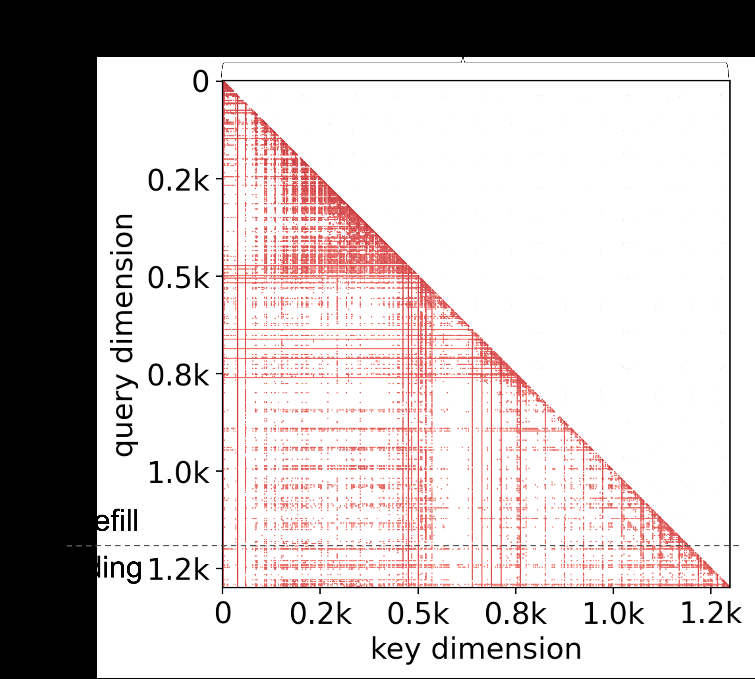
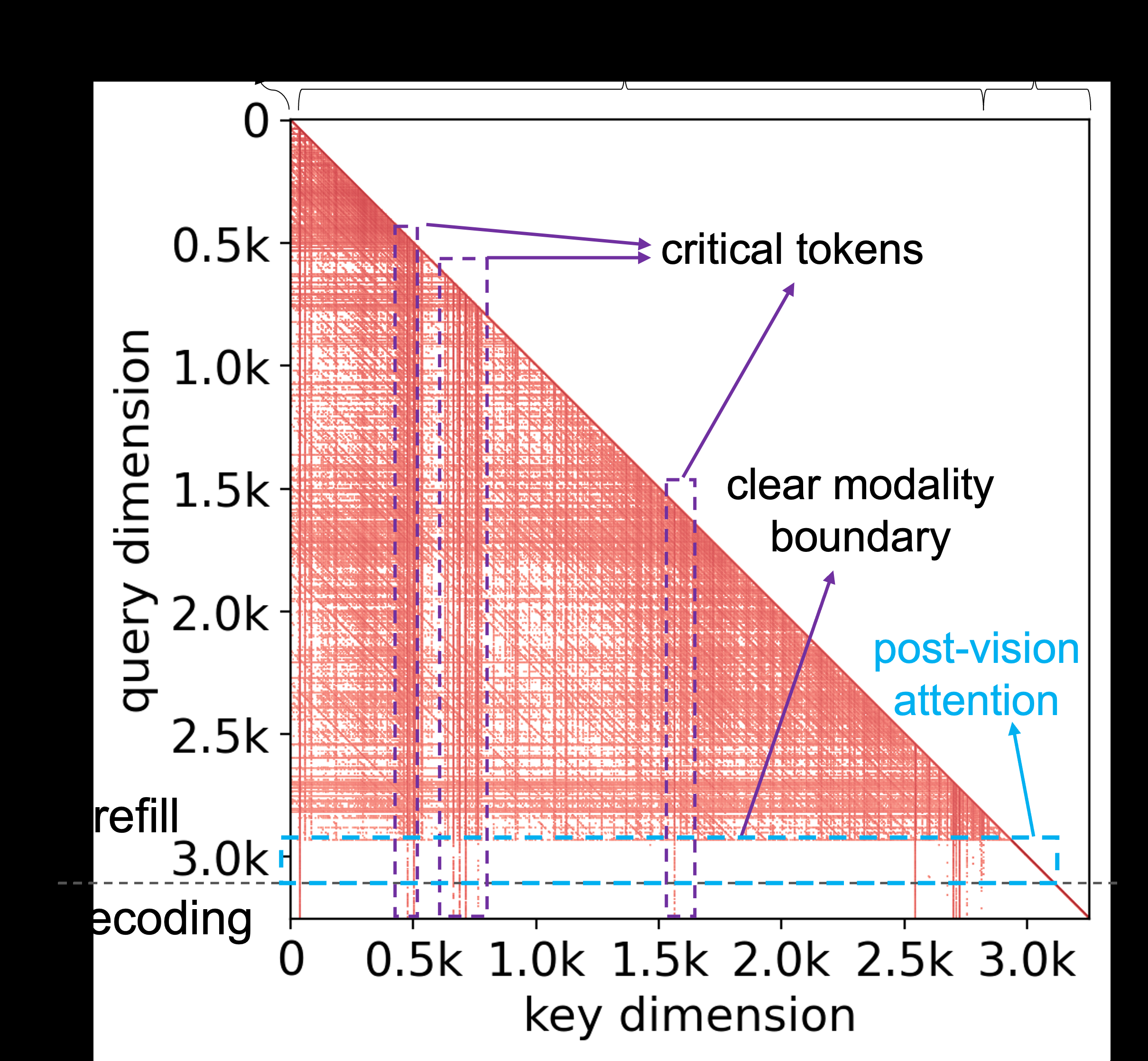
Figure 1 (reproduced above from the paper). Darker red = higher attention score. Both matrices show that the tokens that matter during decoding are largely the same ones that mattered during prefill — which is why KV cache compression is possible at all. The key difference in panel (b) is the clear modality boundary along the query dimension: language tokens attend strongly to the language tokens that come right after the image (the “post-vision” tokens), not diffusely across all preceding visual tokens. This single observation motivates the entire method.
Because prior methods are modality-unaware, they conflate attention mass coming from visual tokens with attention mass coming from language tokens, which — as the paper demonstrates empirically in its accuracy benchmarks (Section 6.2) — leads to suboptimal token eviction decisions for VLMs.
Two more empirical observations that shape the method
- Attention sparsity varies a lot across layers. Measured sparsity ranges from 70% to 99% across transformer layers, with the first couple of layers noticeably denser than the rest. Prior work allocates the same cache budget to every layer (H2O, Keyformer) or a fixed monotonically-decreasing schedule (PyramidKV, PyramidInfer) — both of which under-fit this per-layer variation.
- Sparsity also differs between visual and language tokens, and depends on the specific prompt, so a fixed, prompt-independent budget schedule can’t be optimal — the budget really needs to be computed per prompt, at inference time.
Contributions, restated
- A characterization of VLM attention sparsity across the prefill and decoding phases, showing it’s structurally different from LLM attention.
- Layer-adaptive, sparsity-aware KV cache budget allocation — how much cache each layer gets is computed dynamically from that layer’s own measured sparsity, not from a fixed schedule.
- A modality-aware token scoring policy (“Accumulated Post-vision Attention”) that uses language-to-vision attention as a robust signal for which tokens (visual and language) are worth keeping.
Background
VLM inference: prefill and decoding
Let a VLM prompt be a sequence of m tokens (mixing visual and language tokens after the visual encoder + projection layer have turned image patches into “soft prompt” embeddings): \(\{x_1, \dots, x_m\}\).
Prefill phase. All m tokens are processed in parallel to compute \(P_\theta(x_{m+1} \mid x_1, \dots, x_m)\) — the probability distribution for the first generated token. While doing this, the model caches the per-layer key and value vectors \(\{k_1^{(l)}, \dots, k_m^{(l)}\}\) and \(\{v_1^{(l)}, \dots, v_m^{(l)}\}\) for every transformer layer \(l\), so they don’t need to be recomputed later.
Decoding phase. At step \(i\), the model consumes token \(x_{m+i}\) and computes \(P_\theta(x_{m+i+1} \mid x_1, \dots, x_{m+i})\). This produces new key/value vectors \(k_{m+i}^{(l)}\), \(v_{m+i}^{(l)}\) per layer, which get appended to the running cache. As context length grows (many images, video, or long generations), the KV cache can exceed the size of the model’s own parameters, making memory capacity and bandwidth — not compute — the bottleneck.
KV cache compression: two independent design axes
The paper frames KV cache compression as having exactly two design dimensions, and this framing is the backbone of the whole method:
- Budget allocation — how many cache slots does each layer get?
- Naïve baseline: equal budget per layer (used by StreamingLLM, H2O).
- PyramidKV / PyramidInfer: a fixed, monotonically decreasing budget with depth (more budget to shallow layers, less to deep ones), motivated by the empirical finding that evicting cache at different layers hurts accuracy by different amounts.
- Token scoring policy — which tokens within a layer’s budget get kept?
- Formally: given
ncached tokens at layerlindexed by \(S = \{0, \dots, n\}\), a scoring policy is a function \(\psi: S \to \mathbb{R}^n\). Given a budget \(k \in [1, n)\), the tokens kept are the top-kscorers: \[S_\psi := \{i_1, i_2, \dots, i_k : \psi(S)_{i_j} \ge \psi(S)_{x \in [n]\setminus\{i_1,\dots,i_k\}}\}\] - StreamingLLM keeps only the earliest (“attention sink”) tokens plus the most recent ones.
- H2O uses accumulated attention scores (summed over the query dimension) to keep “heavy hitter” tokens.
- Formally: given
The paper’s unifying insight: KV cache compression only works because transformer attention is sparse in the first place — so both budget allocation and token scoring should be driven by measured sparsity, not fixed heuristics. That idea is developed in the next section.
Preliminary experiments: measuring VLM attention
Before designing the algorithm, the authors run a diagnostic study. They sample prompts from three datasets — DocVQA (OCR/document QA), MathVista (visual math reasoning), and Coco-Caption (captioning, i.e. world knowledge) — feed them through LLaVA-Mistral-7B, and record the full attention score matrices through generation.
Measuring attention sparsity
To measure sparsity cheaply (it needs to run at inference time, not just for offline analysis), the paper defines a fast relative-threshold filter instead of using top-k/top-p truncation (which would require sorting):
\[ \text{ThresholdFilter}(A, p)_{ij} = \begin{cases} A_{ij} & \text{if } A_{ij} \ge p \cdot \max_j(A_{ij}) \\ 0 & \text{otherwise} \end{cases} \qquad (1) \]
with \(p \in (0,1)\) heuristically set to 1% (small enough that the filtered-out scores barely affect the layer’s output). ThresholdFilter is asymptotically faster than top-p/top-k truncation because it doesn’t require sorting the attention distribution.
Given the filtered matrix, per-layer sparsity \(\gamma^{(l)} \in [0,1]\) is the fraction of zero entries in the lower-triangular (causal) portion of the attention matrix:
\[ \gamma^{(l)} := \frac{\sum_{i \ge j} \mathbb{1}[\text{ThresholdFilter}(A^{(l)}, p)_{ij} = 0]}{|\{A_{ij}^{(l)} : i \ge j\}|} \qquad (2) \]
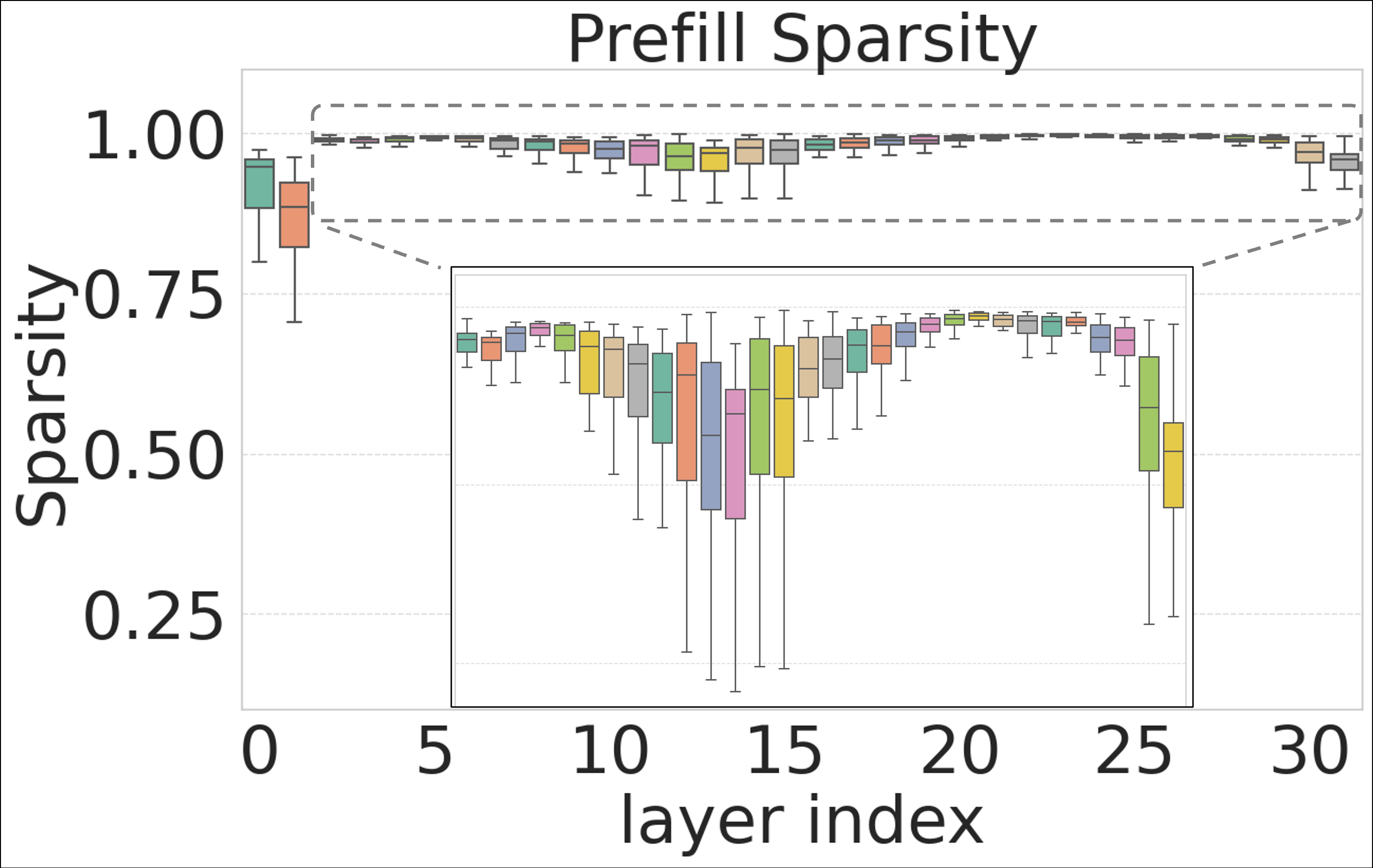
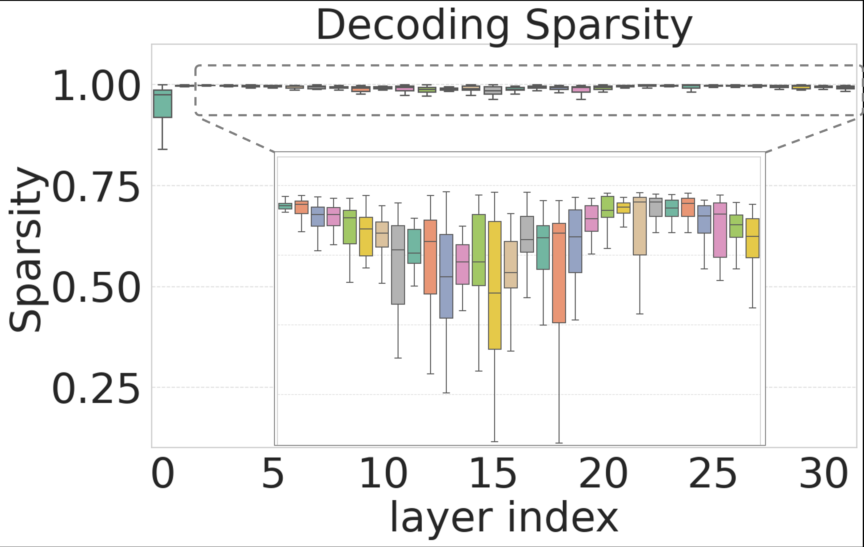
Figure 2 (reproduced from the paper). Each box is one transformer layer’s sparsity distribution (across attention heads and sampled prompts).
Findings from this experiment:
- Sparsity ranges from about 70% to 99% across layers — this is not uniform, contradicting the equal-budget assumption used by H2O/Keyformer.
- The first two layers are noticeably less sparse (denser, more “important” in the sense of needing more cache) than the rest, and a few middle layers are also denser than their neighbors — this non-monotonic pattern contradicts the monotonically decreasing schedule used by PyramidKV/PyramidInfer.
- The decoding-phase sparsity curve (b) closely tracks the prefill-phase curve (a), except the 2nd layer becomes much sparser during decoding. The Pearson correlation coefficient between the prefill and decoding sparsity curves (averaged across layers) is 0.695 — high enough that the authors conclude prefill-phase sparsity can be used to predict how much cache a layer will need during decoding.
This last point is the linchpin of the method: you can measure sparsity once, cheaply, right after prefill, and use it to decide the decoding-phase cache budget — no need to observe decoding attention at all (which wouldn’t be available yet anyway).
Measuring cache hit rate and the “post-vision” hypothesis
Going back to the modality boundary observed in Figure 1(b), the authors hypothesize that scoring cache tokens by their attention from the post-vision language tokens (rather than from the whole prompt) will more faithfully identify which tokens the model actually needs during decoding.
To test this rigorously, they define an oracle-relative metric.
Let \(m\) be the prompt length, \(Q_{:m}, K_{:m} \in \mathbb{R}^{m \times d}\) the query/key matrices, and \(Q_{m+1} \in \mathbb{R}^d\) the query vector of the first decoded token. Define the true decoding-time attention distribution:
\[A_{m+1} := \text{softmax}\!\left(\frac{Q_{m+1} K_{:m}^T}{\sqrt d}\right) \in \mathbb{R}^m\]
- \(\psi^*: S \to A_{m+1}\) — the optimal scoring function (uses the real decoding attention — only observable in hindsight).
- \(S_{\psi^*}\) — the top-
ktokens under \(\psi^*\) (optimal for any budgetk). - CacheHitRate \(:= \dfrac{|S_\psi \cap S_{\psi^*}|}{|S_{\psi^*}|}\) — the fraction of the true important tokens that a practical (prefill-only) policy \(\psi\) actually manages to keep.
Since \(A_{m+1}\) is only known after decoding starts — and the entire point of compression is to shrink the cache before decoding — multiple prefill-time approximations \(\psi\) have been proposed:
| Policy | Definition | Idea |
|---|---|---|
| Accumulated Attention (prior work, e.g. H2O) | \(\psi(S) := \sum_i \text{softmax}\!\left(\frac{Q_{:m}K_{:m}^T}{\sqrt d}\right)_i\) | Sum attention over the entire query dimension. |
| Accumulated Sliding Window Attention (prior work) | \(\psi(S) := \sum_i \text{softmax}\!\left(\frac{Q_{m-w:m}K_{m-w:m}^T}{\sqrt d}\right)_i\) | Sum only over a fixed-size recent window \(w\). |
| Accumulated Post-vision Attention (this paper) | \(\psi(S) := \sum_i \text{softmax}\!\left(\frac{Q_{m-\tau:m}K_{m-\tau:m}^T}{\sqrt d}\right)_i\) | Sum only over the \(\tau\) language tokens that follow the vision tokens in the prompt. |
τ is the count of language tokens that follow the vision tokens in the prompt — so Accumulated Post-vision Attention is a dynamic, prompt-dependent sliding window, where the window size is exactly the length of the post-vision language prompt, instead of a fixed, hand-tuned w.
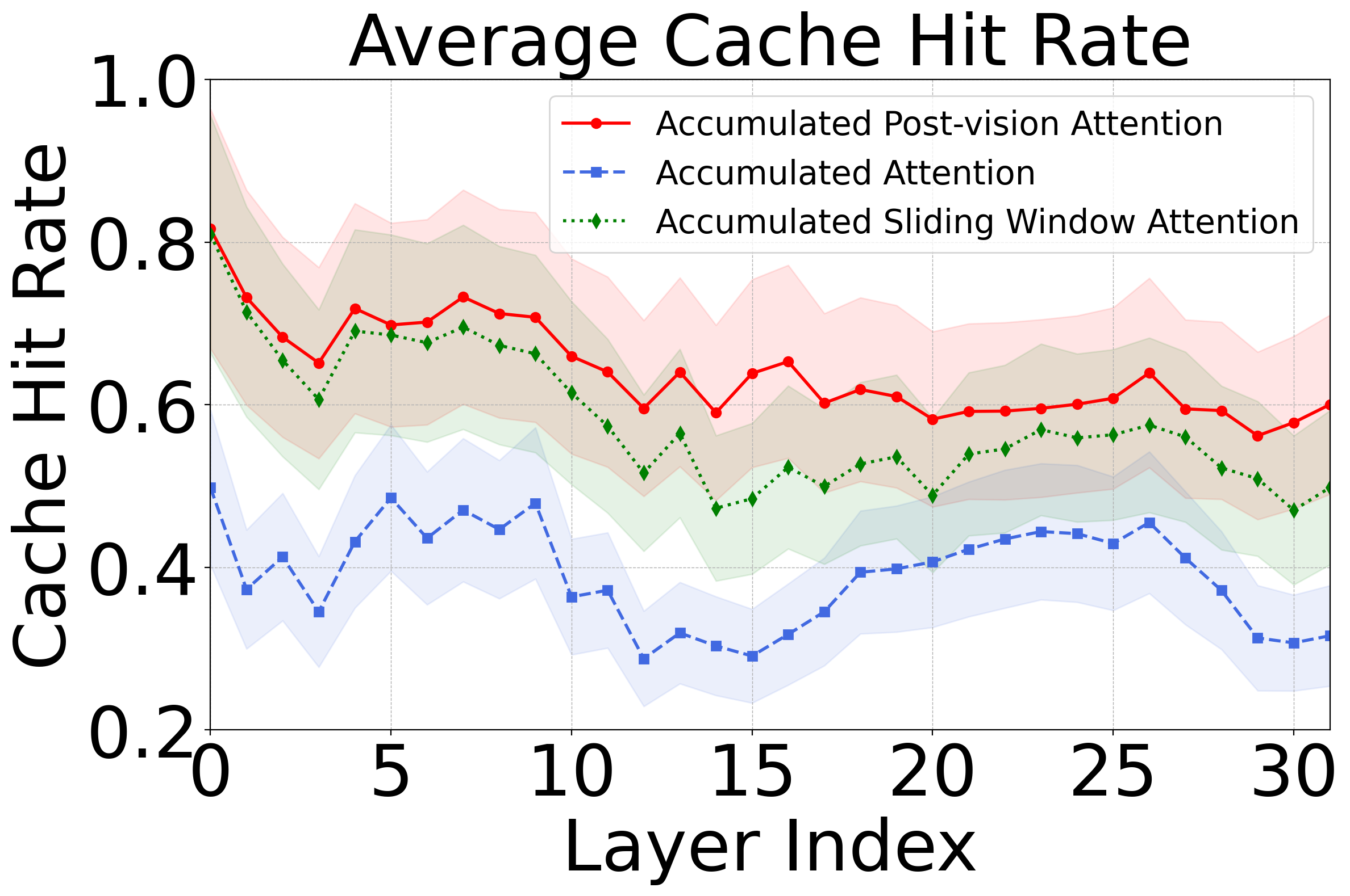
Why does plain Accumulated Attention do worse? Summing over the entire query dimension unavoidably gives high scores to early tokens simply because more queries have had the chance to attend to them — a length bias. A sliding window helps, but a fixed window size is a blunt instrument: it can be too large or too small depending on how long the post-vision prompt happens to be for a given input. Post-vision Attention sidesteps this by letting the “window” be exactly the post-vision language span, which is exactly where the modality boundary in Figure 1(b) shows the useful signal concentrating.
The VL-Cache method
VL-Cache combines the two findings above into a two-stage recipe that runs almost entirely during the prefill phase (so its cost is a one-time overhead amortized over many decoding steps):
- Use Post-vision Attention to compute per-layer sparsity, and turn that into a per-layer cache budget.
- Use the same Post-vision Attention matrix to score and keep the top-
ktokens within each layer’s allotted budget.
The paper denotes the Post-vision Attention matrix \(A'\) for brevity throughout this section.
flowchart TB
    PVA["Prefill stage — compute Post-vision Attention A′<br/>(query window = last τ post-vision tokens)"]:::prefill
    SPARSE["Prefill stage — sparsity-aware budget allocation<br/>score_j := Σᵢ A′ᵢⱼ  →  per-layer sparsity γ′⁽ˡ⁾  →  budget β⁽ˡ⁾"]:::prefill
    PVA --> SPARSE
    SPARSE -->|"shrink KV cache size / score token significance"| DSI

    DSI(["Decoding step i"]) -- "q_i⁰" --> L0["Layer 0 — Key/Value cache<br/>(β⁽⁰⁾ tokens kept: visual + language)"]:::decode
    L0 -- "q_i¹" --> L1["Layer 1 — Key/Value cache<br/>(β⁽¹⁾ tokens kept)"]:::decode
    L1 -. "…" .-> LN["Layer N — Key/Value cache<br/>(β⁽ᴺ⁾ tokens kept)"]:::decode
    LN -- "q_iᴺ" --> DSI2(["Decoding step i+1"])

    classDef prefill fill:#fbe1e1,stroke:#a33,color:#111,stroke-width:1px
    classDef decode fill:#dde9f8,stroke:#357,color:#111,stroke-width:1px
Figure 4, redrawn as Mermaid (original: “VL-Cache Overview”, page 6 of the paper — see also the original raster inset for the attention-heatmap icon used in the paper’s version). In the prefill stage, the cache budget for every layer is set dynamically from that layer’s own Post-vision-Attention sparsity; then, still using Post-vision Attention, both critical visual tokens and language tokens are selected to fill each layer’s budget before decoding starts.
Sparsity-aware KV cache budget allocation
Two steps happen once, right after prefill:
- Apply
ThresholdFilter(with \(p = 1\%\)) to the Post-vision Attention scores \(A'\) and compute layer-wise sparsity \(\gamma'^{(l)}\) (same recipe as Eq. 1–2, but restricted to the post-vision query rows). - Given a global target cache budget \(\alpha\) (a hyperparameter — e.g. \(\alpha = 10\%\) means “keep 10% of the KV cache overall”), distribute that budget across layers in proportion to each layer’s density (i.e. \(1 - \gamma'^{(l)}\)): sparser layers get less cache, denser layers get more.
Input:  query and key Q, K ∈ R^(L×H×m×d), number of layers L,
        number of heads H, length of post-vision prompt τ,
        cache budget α.
Output: layer-wise budget β

procedure ComputeSparsity(Q, K):
    Q' ← Q[m-τ:m]
    A' ← softmax(Q' Kᵀ / √d)
    γ' ← Σ_{i+m-τ≥j} 1[ThresholdFilter(A', p)_ij = 0]
         ─────────────────────────────────────────────
                    |{A'_ij : i+m-τ ≥ j}|
    return γ'

procedure SkewedCacheBudgetAllocation(Q, K, α, L, H):
    Γ[L][H] ← 0
    for l = 1 → L:
        for h = 1 → H:
            Γ[l][h] ← ComputeSparsity(Q_h^(l), K_h^(l))
    γ' ← Γ.mean(axis=1)                 # average over heads
    Z  ← Σ_l (1 − γ'^(l))
    β[L] ← 0
    for l = 1 → L:
        β^(l) ← clip( (1 − γ'^(l)) / Z · αL ,  0.01,  1 )
    return β
The same logic, as a flowchart:
flowchart TD
    START(["Input: Q, K ∈ ℝ^(L×H×m×d)<br/>layers L, heads H, post-vision length τ, budget α"]) --> OUTER{"for layer l = 1…L"}
    OUTER --> INNER{"for head h = 1…H"}
    INNER --> CS["ComputeSparsity(Qₕ⁽ˡ⁾, Kₕ⁽ˡ⁾):<br/>Q′ = Q[m−τ:m]<br/>A′ = softmax(Q′Kᵀ/√d)<br/>γ′ = fraction of ThresholdFilter(A′,p) = 0<br/>in the post-vision causal region"]
    CS --> INNER
    INNER -->|all heads done| OUTER
    OUTER -->|all layers done| AGG["γ′⁽ˡ⁾ = mean over heads<br/>Z = Σₗ (1 − γ′⁽ˡ⁾)"]
    AGG --> ALLOC["for layer l = 1…L:<br/>β⁽ˡ⁾ = clip( (1−γ′⁽ˡ⁾)/Z · αL , 0.01, 1 )"]
    ALLOC --> RET(["Return per-layer budget β"])
Key contrast with PyramidKV: PyramidKV uses one fixed monotonically-decreasing budget schedule for every prompt. VL-Cache’s \(\beta^{(l)}\) is recomputed per prompt from that prompt’s own measured sparsity pattern — so a document-heavy prompt and a short-caption prompt get different per-layer allocations, instead of being forced into the same static shape. Note the allocation is only computed once, immediately after prefill, so its cost is amortized over the (potentially many) subsequent decoding steps.
Modality-aware token scoring policy
Once each layer knows its budget \(k^{(l)}\) (the token count implied by \(\beta^{(l)}\)), VL-Cache still needs to decide which \(k^{(l)}\) tokens to keep. It reuses the same Post-vision Attention matrix \(A'\) (Accumulated Post-vision Attention from Section 4.2) as the scoring function.
Two advantages are argued for reusing Post-vision Attention here, rather than the full attention matrix used by prior work (e.g. H2O):
- Efficiency. Computing layer-wise sparsity/scores from Post-vision Attention costs \(O(\tau m)\) instead of \(O(m^2)\) for the full attention matrix — because \(\tau \ll m\) for realistic vision-language prompts (the post-vision instruction/question is typically much shorter than the full prompt, which is dominated by visual tokens).
- Better token preservation. As shown empirically in Figure 3 (Section 4.2), Post-vision Attention achieves a higher CacheHitRate than plain Accumulated Attention or a fixed sliding window, i.e. it more reliably keeps the tokens that the model will actually attend to during decoding.
The narrative tying it together: plain Accumulated Attention over-weights early tokens (length bias); a fixed sliding window helps but its size is a poorly-chosen constant across very different prompts; Post-vision Attention is a prompt-adaptive sliding window whose size is derived from the prompt’s own structure (the post-vision span), which is exactly where the paper’s Figure 1(b) modality-boundary observation says the useful signal lives.
Experiments
Setup
| Model | Visual model | Language model | Attention type |
|---|---|---|---|
llava-v1.6-mistral-7b |
openai/clip-vit-large-patch14-336 |
Mistral-7B-Instruct-v0.2 | GQA (Grouped Query Attention) |
llava-v1.6-34b |
openai/clip-vit-large-patch14-336 |
Nous-Hermes-2-Yi-34B | MHA (Multi-Head Attention) |
- Hardware: AWS EC2 P4 instance, 8× A100 40GB GPUs.
- Tasks (via
lmms-eval): Coco-Caption (metric: CIDEr — captioning / world knowledge), DocVQA (metric: ANLS — document OCR/QA), MathVista (metric: ACC — visual math reasoning). - Baselines: full KV cache, StreamingLLM, H2O, PyramidKV — all configured with default settings, budget scaled proportionally to prompt length, and recent-token window fixed at 10% of the budget for a fair comparison.
Accuracy evaluation
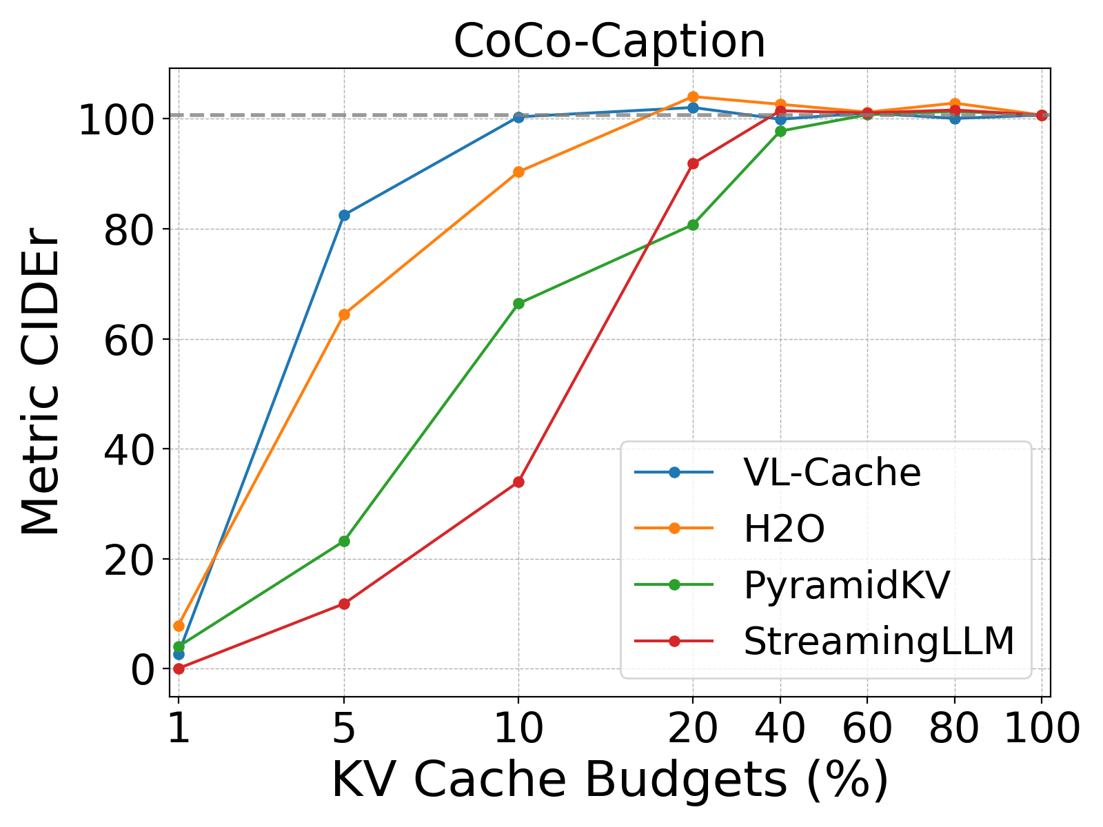
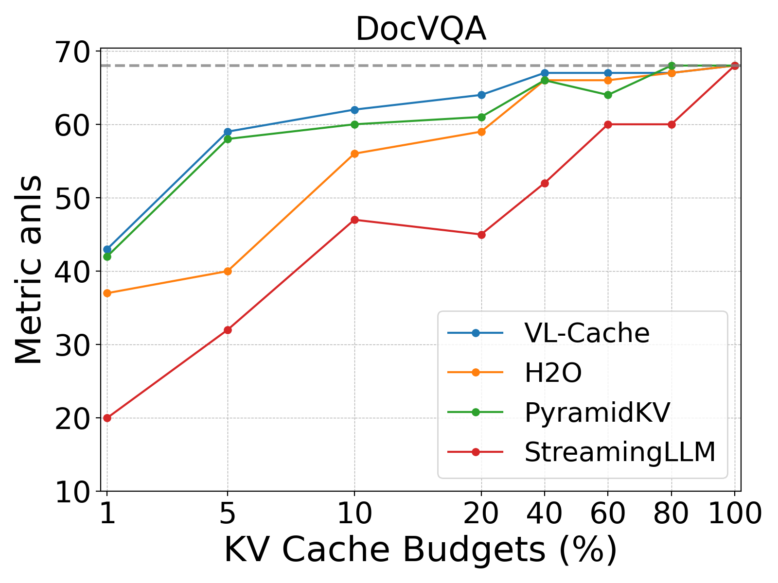
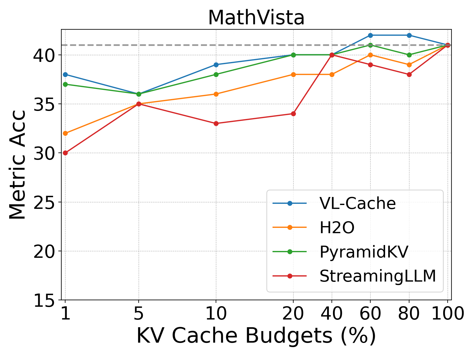
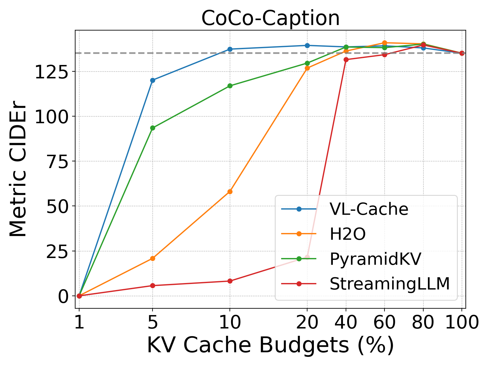
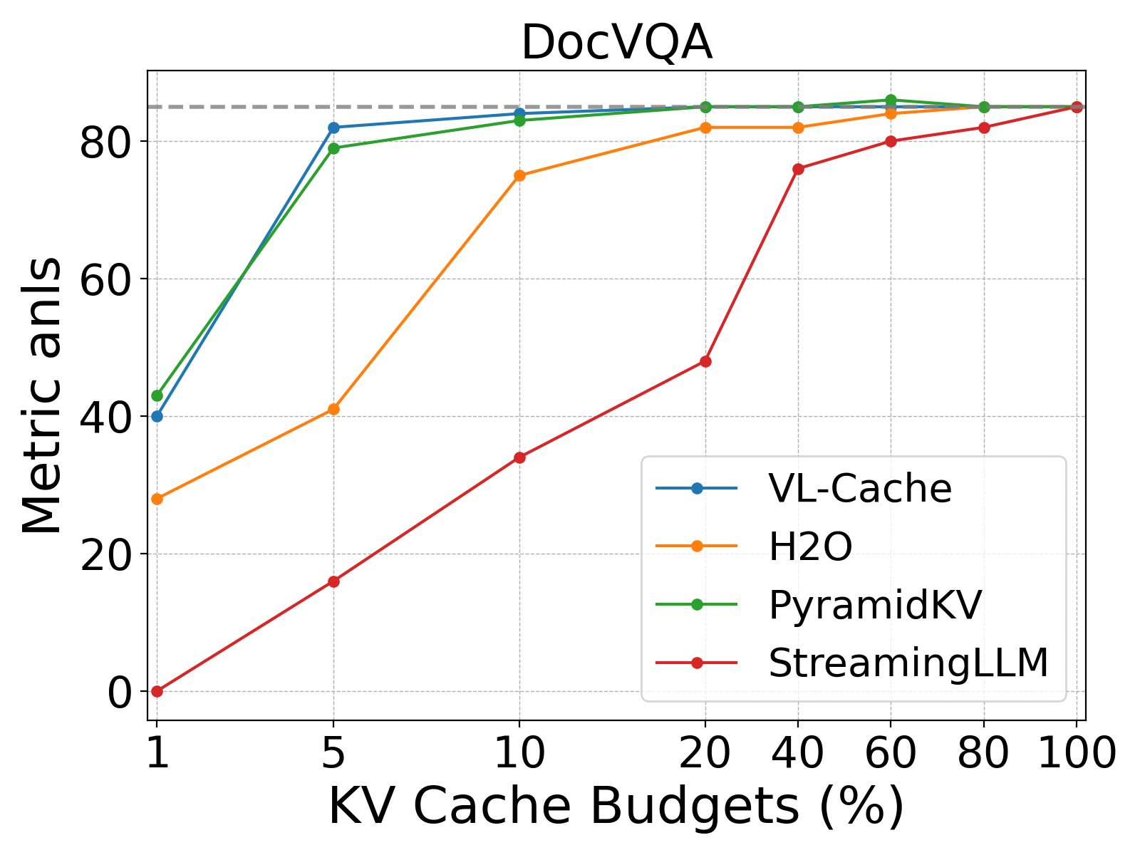
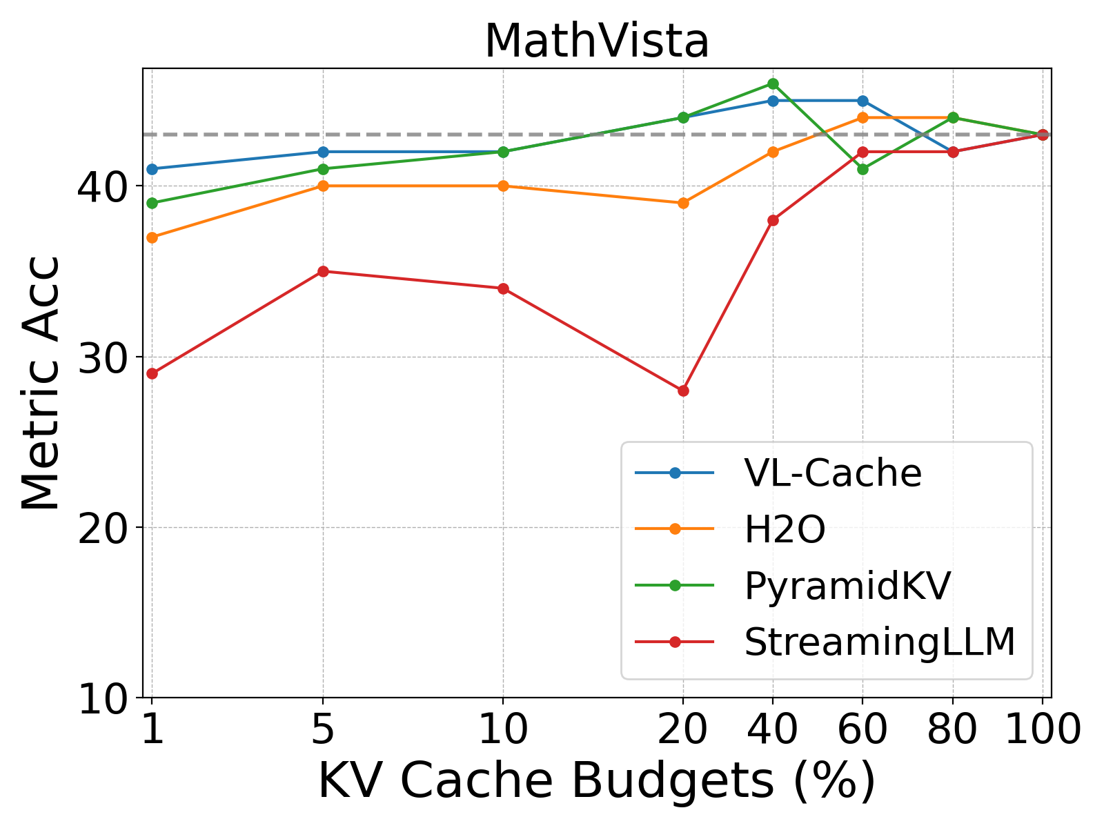
Figure 5 (reproduced from the paper). Accuracy vs. KV cache budget (1–100% of prompt length), for both LLaVA backbones across all three datasets. The dashed grey line marks full-cache accuracy.
Full accuracy table
| Dataset (metric) | Model | Method | 1% | 5% | 10% | 20% | 40% | 60% | 80% | 100% |
|---|---|---|---|---|---|---|---|---|---|---|
| Coco-Caption (CIDEr) | LLaVA-Mistral-7B | VL-Cache | 2.64 | 82.53 | 100.36 | 102.06 | 99.93 | 101.07 | 100.08 | 100.68 |
| H2O | 7.87 | 64.45 | 90.36 | 104.04 | 102.64 | 101.21 | 102.86 | 100.68 | ||
| PyramidKV | 4.01 | 23.21 | 66.41 | 80.76 | 97.76 | 100.75 | 101.38 | 100.68 | ||
| StreamingLLM | 0.05 | 11.82 | 33.98 | 91.87 | 101.47 | 101.07 | 101.6 | 100.68 | ||
| Coco-Caption (CIDEr) | LLaVA-1.6-34B | VL-Cache | 0 | 120.11 | 137.35 | 139.42 | 138.58 | 139.19 | 138.01 | 135.07 |
| H2O | 0 | 20.87 | 58.14 | 126.8 | 136.27 | 140.89 | 140.3 | 135.07 | ||
| PyramidKV | 0 | 93.47 | 116.91 | 129.59 | 138.53 | 138.17 | 140.15 | 135.07 | ||
| StreamingLLM | 0 | 5.69 | 8.23 | 21.57 | 131.51 | 134.26 | 139.65 | 135.07 | ||
| DocVQA (ANLS) | LLaVA-Mistral-7B | VL-Cache | 43 | 59 | 62 | 64 | 67 | 67 | 67 | 68 |
| H2O | 37 | 40 | 56 | 59 | 66 | 66 | 67 | 68 | ||
| PyramidKV | 42 | 58 | 60 | 61 | 66 | 64 | 68 | 68 | ||
| StreamingLLM | 20 | 32 | 47 | 45 | 52 | 60 | 60 | 68 | ||
| DocVQA (ANLS) | LLaVA-1.6-34B | VL-Cache | 41 | 82 | 84 | 85 | 85 | 85 | 85 | 85 |
| H2O | 28 | 41 | 75 | 82 | 82 | 84 | 85 | 85 | ||
| PyramidKV | 43 | 79 | 83 | 85 | 85 | 86 | 85 | 85 | ||
| StreamingLLM | 0 | 16 | 34 | 48 | 76 | 80 | 82 | 85 | ||
| MathVista (ACC) | LLaVA-Mistral-7B | VL-Cache | 38 | 36 | 39 | 40 | 40 | 42 | 42 | 41 |
| H2O | 32 | 35 | 36 | 38 | 38 | 40 | 39 | 41 | ||
| PyramidKV | 37 | 36 | 38 | 40 | 40 | 41 | 40 | 41 | ||
| StreamingLLM | 30 | 35 | 33 | 34 | 40 | 39 | 38 | 41 | ||
| MathVista (ACC) | LLaVA-1.6-34B | VL-Cache | 41 | 42 | 42 | 44 | 45 | 45 | 42 | 43 |
| H2O | 37 | 40 | 40 | 39 | 42 | 44 | 44 | 43 | ||
| PyramidKV | 39 | 41 | 42 | 44 | 46 | 41 | 44 | 43 | ||
| StreamingLLM | 29 | 35 | 34 | 28 | 38 | 42 | 42 | 43 |
Reading the results:
- Coco-Caption: all baselines are fine once the budget exceeds ~40%, but degrade sharply below that. VL-Cache is the standout at the low end — 5–10% budget is already comparable to a full cache. H2O and StreamingLLM (equal budget per layer) miss important tokens in dense layers while wasting budget in sparse ones; PyramidKV’s fixed monotonic schedule is “ineffective for all input queries” per the authors.
- DocVQA: PyramidKV is the strongest baseline here, but VL-Cache still consistently comes out ahead across the whole budget range. H2O and StreamingLLM again lack robustness as the budget shrinks.
- MathVista: differences are smaller in absolute terms (the task appears less sensitive to cache budget generally) but VL-Cache remains competitive to best-in-class across budgets.
Speed benchmark
Latency is measured as raw GPU kernel time (via PyTorch Profiler) using synthetic prompts of increasing length (1K → 128K tokens) and batch sizes (1 → 64), following the benchmarking methodology of vLLM’s PagedAttention paper (Kwon et al., 2023). The baseline uses HuggingFace’s default implementation with FlashAttention-v2; VL-Cache uses custom Triton kernels (detailed in Section 8.3) for the attention-statistics pass. Speedup is always baseline latency / VL-Cache latency.
| Batch size | Prompt length | Prefill speedup | Decoding speedup | End-to-end speedup |
|---|---|---|---|---|
| 1 | 2,000 | 0.96 | 1.19 | 1.16 |
| 1 | 8,000 | 0.97 | 1.70 | 1.49 |
| 1 | 32,000 | 0.99 | 3.32 | 1.85 |
| 1 | 128,000 | 0.99 | 7.08 | 1.66 |
| 4 | 2,000 | 0.98 | 1.68 | 1.50 |
| 4 | 8,000 | 0.98 | 3.16 | 1.95 |
| 4 | 32,000 | 0.99 | 6.07 | 2.06 |
| 16 | 2,000 | 0.98 | 3.03 | 1.99 |
| 16 | 8,000 | 0.99 | 5.61 | 2.27 |
| 64 | 2,000 | 0.98 | 5.23 | 2.33 |
How to read these numbers:
- Prefill is barely affected (speedup ≈ 0.96–0.99, i.e. essentially neutral, occasionally a hair slower) — this is expected, since the extra attention-statistics computation is small and happens only once per request; Appendix A.4 shows it’s just 1–6% overhead on top of prefill latency, shrinking further as prompts get longer.
- Decoding speedup grows with prompt length, reaching 7.08× at 128K tokens/batch 1 — because that’s exactly where a smaller KV cache saves the most HBM traffic per decoding step.
- End-to-end speedup is bounded above by decoding speedup, since prefill is unaffected. At 128K tokens/batch 1, decoding is 7.08× faster, but prefill still eats 53% of total latency, so the blended end-to-end number comes out to only 1.66×. As the number of output tokens generated grows, end-to-end speedup asymptotically approaches the decoding speedup — meaning VL-Cache is most valuable for long-output tasks: captioning, video description, chain-of-thought multi-modal reasoning, etc.
- Because batch size in this setup is capped by peak prefill memory, not KV cache size, compression here doesn’t directly raise the maximum batch size — the authors note that continuous batching / chunked prefill (future work) would let KV-cache size become the binding constraint, at which point VL-Cache’s memory savings would translate into higher concurrency too.
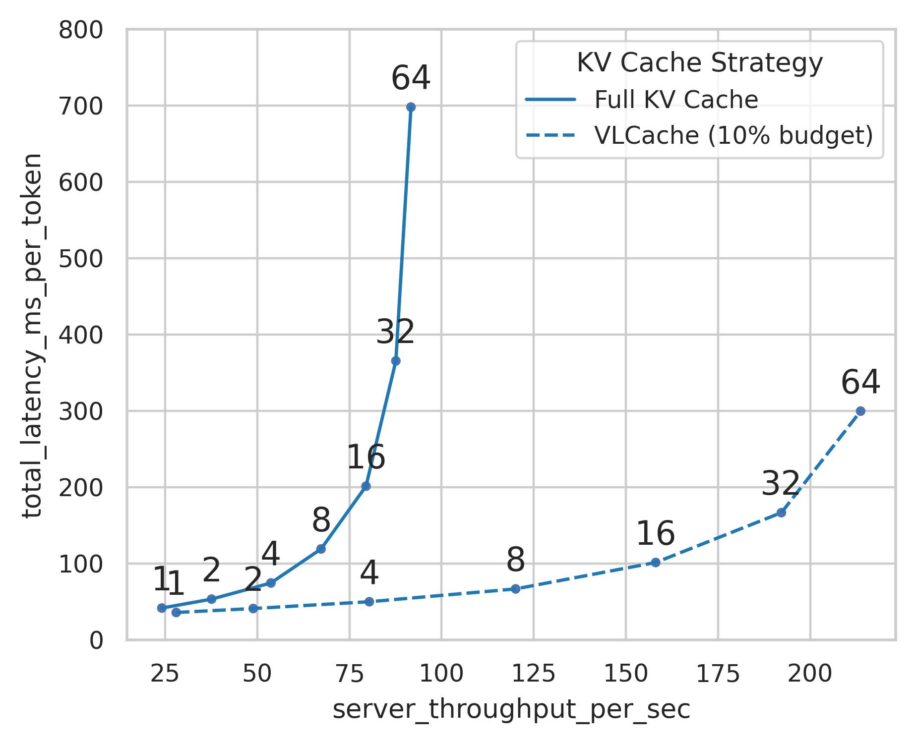
- Figure 6 shows the practical payoff for a server operator: at any given target latency, VL-Cache serves noticeably higher throughput than the full-cache baseline, and vice versa — for the same throughput target, requests see lower latency.
Conclusion
VL-Cache is a KV-cache compression method purpose-built for VLMs, built on two empirical observations: (1) attention sparsity varies substantially and non-monotonically across transformer layers, and this can be measured cheaply during prefill and used to predict decoding-time cache needs; and (2) VLM attention has a modality boundary, and language-to-post-vision attention is a robust, efficient signal for scoring token importance for both visual and language tokens. Combining a sparsity-aware, per-prompt, per-layer budget allocation with a modality-aware (“Accumulated Post-vision Attention”) token scoring policy, VL-Cache retains accuracy comparable to a full KV cache while keeping only 10% of it, and delivers up to 2.33× end-to-end and 7.08× decoding speedups.
Appendix
A.1 — Vision-language prompt template construction
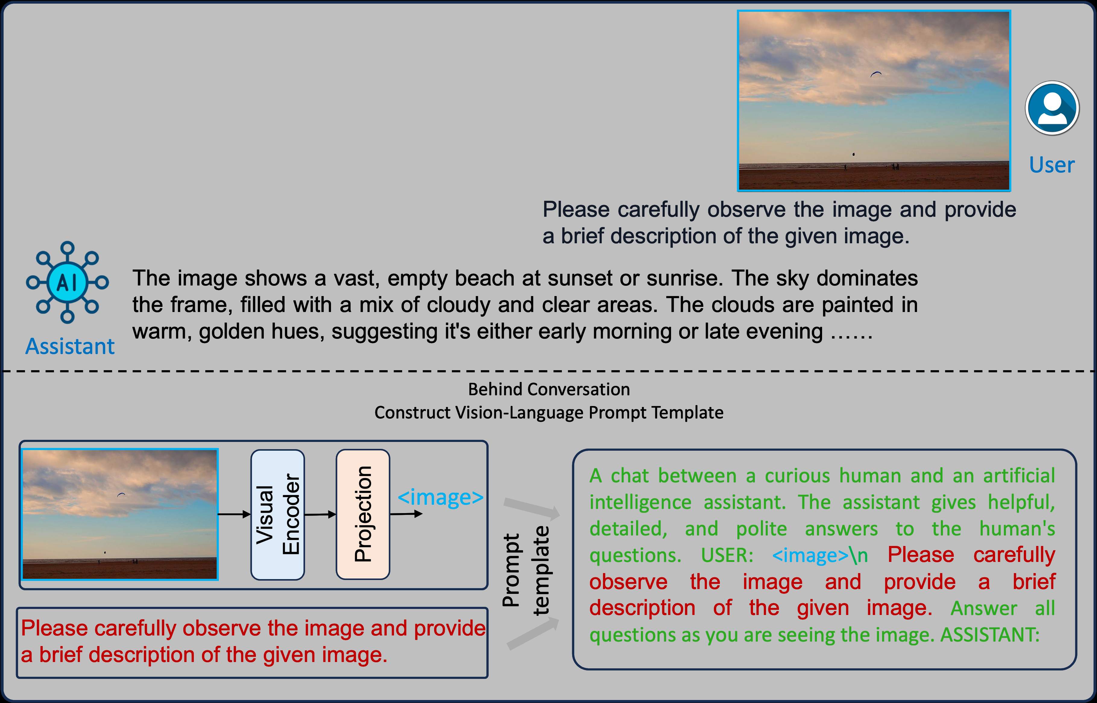
<image> embedding, then combined with a system/user prompt template.The point of this figure is subtle but important for why VL-Cache’s Post-vision Attention signal is robust: standard VLM prompt-template conventions (used across LLaVA, Gemini, GPT-4o, Qwen-VL, Claude, etc.) mean that regardless of whether the image appears before or after the user’s text in the raw conversation, the templated prompt fed to the model always places a language-based instruction or question in the post-vision position. That’s what makes “the last τ tokens after the vision block” a reliable, prompt-independent way to locate the useful signal — it doesn’t require knowing anything about how the user phrased their input.
The underlying process, generalized as a flow:
flowchart TB
IMG["Input image"] --> VE["Visual encoder<br/>(e.g. CLIP ViT-L/14-336)"]
VE --> PROJ["Projection layer (MLP)"]
PROJ --> IMGEMB["<image> embedding<br/>(soft prompt tokens)"]
USERTXT["User instruction / question<br/>(may precede or follow the<br/>image in the raw conversation)"]
SYS["System / conversation<br/>prompt template"]
IMGEMB --> COMBINE["Templated prompt:<br/>system + <image> + instruction"]
USERTXT --> COMBINE
SYS --> COMBINE
COMBINE --> POSTVISION["Post-vision language span (length τ)<br/>always right after <image>,<br/>regardless of original ordering"]
POSTVISION --> LM["Language model"]
LM --> OUT["Generated response"]
A.2 — Extended related work
A.3 — Efficient implementation (Triton kernels)
To find low-attention tokens during prefill without blowing the latency/memory budget, VL-Cache needs two statistics computed from the (potentially huge) attention score matrix:
- The average attention score per token in the key dimension (used for token scoring).
- The count of attention scores below
p% of the row maximum, in the query dimension (used for the sparsity ratio, per Eq. 1–2).
The catch: modern fused-attention kernels like FlashAttention and PagedAttention deliberately never materialize the full attention score matrix in HBM (that’s exactly what makes them fast). So VL-Cache needs a new, similarly memory-efficient kernel that computes these two statistics without ever writing the full attention matrix back to HBM. The design constraints, verbatim from the paper:
- The attention mask is not written to HBM.
- The \(QK^T\) product is not written to HBM.
- The attention scores are not written to HBM.
- Similarly-parallelized elementwise operations (e.g. division, addition) are fused to avoid intermediate tensors in HBM.
Their first attempt — torch.compile with the Triton backend — satisfied constraints (1), (3), and (4), but not (2): it could not automatically discover the fused matmul+softmax trick that FlashAttention uses (partitioning work along the Q dimension, keeping one Q tile resident in SRAM, and streaming K/V tiles through it while running an online softmax). So they hand-wrote the fused kernel in Triton.
The wrinkle for the second statistic (average attention per token in the K dimension) is that it requires reducing over the query dimension — the opposite axis from what the fused matmul+softmax kernel already partitions over. That forces a second kernel, partitioned over K instead of Q, which has to recompute softmax (since the scores were never stored) — but it can reuse the row-wise max/sum tensors the first kernel already computed and stored (both only \(O(Q)\) in size, so cheap to keep in HBM).
flowchart TD
    IN["Q, K in HBM"] --> K1["Kernel 1 — Softmax + row-wise stats<br/>(reduction over K dim, Q-dim partitioned, online softmax)<br/>• pre-exp max over K (numerical stability)<br/>• post-exp sum over K (softmax normalizer)"]
    K1 -->|"pre-exp max, post-exp sum<br/>(both O(Q), written to HBM)"| K2["Kernel 2 — Softmax + column-wise stats<br/>(reduction over Q dim, K-dim partitioned;<br/>re-derives softmax from Kernel 1's stats)<br/>• post-softmax sum over Q → avg. attention/token<br/>• count of scores below p·max over Q → sparse count"]
    K2 -->|"partial sparse-count per thread block"| K3["Kernel 3 — Sum reduction<br/>of partial sparse counts"]
    K3 --> OUT["Attention statistics:<br/>avg. attention score / token (scoring)<br/>+ per-layer sparsity ratio (budget allocation)"]
The authors report that each of their two hand-written Triton kernels has roughly the same latency as a FlashAttention kernel — evidence that the 3-kernel partitioning is close to optimal for this problem. Given that overhead, they note the practical need to keep the number of query tokens used for statistics small (their benchmark uses only the last 50 tokens of the prompt).
A.4 — Detailed speed benchmark results
Measured with PyTorch Profiler (summing GPU-kernel latencies only, excluding CPU-side overhead not attributable to the method). Blank cells indicate the inference server ran out of GPU memory during prefill at that batch size / prompt length combination.
Prefill overhead — cumulative latency (ms) of computing attention statistics (50 query tokens), eviction scores for all prompt tokens, and copying the post-eviction (90%-compressed) KV cache into contiguous memory:
| Batch size | 1,000 | 2,000 | 4,000 | 8,000 | 16,000 | 32,000 | 64,000 | 128,000 |
|---|---|---|---|---|---|---|---|---|
| 1 | 5.20 | 7.20 | 10.10 | 17.30 | 28.30 | 49.70 | 100.20 | 189.60 |
| 2 | 6.40 | 9.50 | 15.80 | 29.00 | 51.80 | 92.50 | 188.50 | – |
| 4 | 8.50 | 15.20 | 27.40 | 52.50 | 93.30 | 175.80 | – | – |
| 8 | 13.70 | 26.80 | 50.90 | 96.60 | 178.40 | – | – | – |
| 16 | 25.20 | 51.30 | 95.60 | 183.50 | – | – | – | – |
| 32 | 48.50 | 97.10 | 182.60 | – | – | – | – | – |
| 64 | 91.60 | 186.70 | – | – | – | – | – | – |
Prefill speedup — ratio \(\frac{\text{prefill}}{\text{prefill} + \text{overhead}}\) (i.e. how much prefill latency the statistics overhead “costs”; values below 1.0 indicate overhead, never more than 6%, and it shrinks as prompts get longer):
| Batch size | 1,000 | 2,000 | 4,000 | 8,000 | 16,000 | 32,000 | 64,000 | 128,000 |
|---|---|---|---|---|---|---|---|---|
| 1 | 0.94 | 0.96 | 0.97 | 0.97 | 0.99 | 0.99 | 0.99 | 0.99 |
| 2 | 0.96 | 0.97 | 0.97 | 0.98 | 0.98 | 0.99 | 0.99 | – |
| 4 | 0.97 | 0.98 | 0.98 | 0.98 | 0.98 | 0.99 | – | – |
| 8 | 0.98 | 0.98 | 0.98 | 0.99 | 0.99 | – | – | – |
| 16 | 0.98 | 0.98 | 0.99 | 0.99 | – | – | – | – |
| 32 | 0.98 | 0.98 | 0.98 | – | – | – | – | – |
| 64 | 0.99 | 0.98 | – | – | – | – | – | – |
Decoding speedup — ratio of decoding latency with a full KV cache vs. decoding latency with a 10%-of-prompt-length KV cache:
| Batch size | 1,000 | 2,000 | 4,000 | 8,000 | 16,000 | 32,000 | 64,000 | 128,000 |
|---|---|---|---|---|---|---|---|---|
| 1 | 1.10 | 1.19 | 1.37 | 1.70 | 2.31 | 3.32 | 5.17 | 7.08 |
| 2 | 1.18 | 1.36 | 1.68 | 2.27 | 3.16 | 4.56 | 6.78 | – |
| 4 | 1.36 | 1.68 | 2.26 | 3.16 | 4.39 | 6.07 | – | – |
| 8 | 1.73 | 2.29 | 3.13 | 4.37 | 5.87 | – | – | – |
| 16 | 2.19 | 3.03 | 4.18 | 5.61 | – | – | – | – |
| 32 | 2.94 | 4.12 | 5.53 | – | – | – | – | – |
| 64 | 3.83 | 5.23 | – | – | – | – | – | – |
End-to-end speedup — ratio of full-cache baseline latency to VL-Cache latency, where VL-Cache latency includes prefill + overhead + 99 decoding passes (100 output tokens total):
| Batch size | 1,000 | 2,000 | 4,000 | 8,000 | 16,000 | 32,000 | 64,000 | 128,000 |
|---|---|---|---|---|---|---|---|---|
| 1 | 1.09 | 1.16 | 1.30 | 1.49 | 1.71 | 1.85 | 1.89 | 1.66 |
| 2 | 1.16 | 1.30 | 1.49 | 1.73 | 1.89 | 1.97 | 1.94 | – |
| 4 | 1.30 | 1.50 | 1.74 | 1.95 | 2.06 | 2.06 | – | – |
| 8 | 1.54 | 1.79 | 2.00 | 2.17 | 2.23 | – | – | – |
| 16 | 1.75 | 1.99 | 2.17 | 2.27 | – | – | – | – |
| 32 | 1.98 | 2.19 | 2.32 | – | – | – | – | – |
| 64 | 2.18 | 2.33 | – | – | – | – | – | – |
A.5 — Measuring attention to visual vs. language tokens
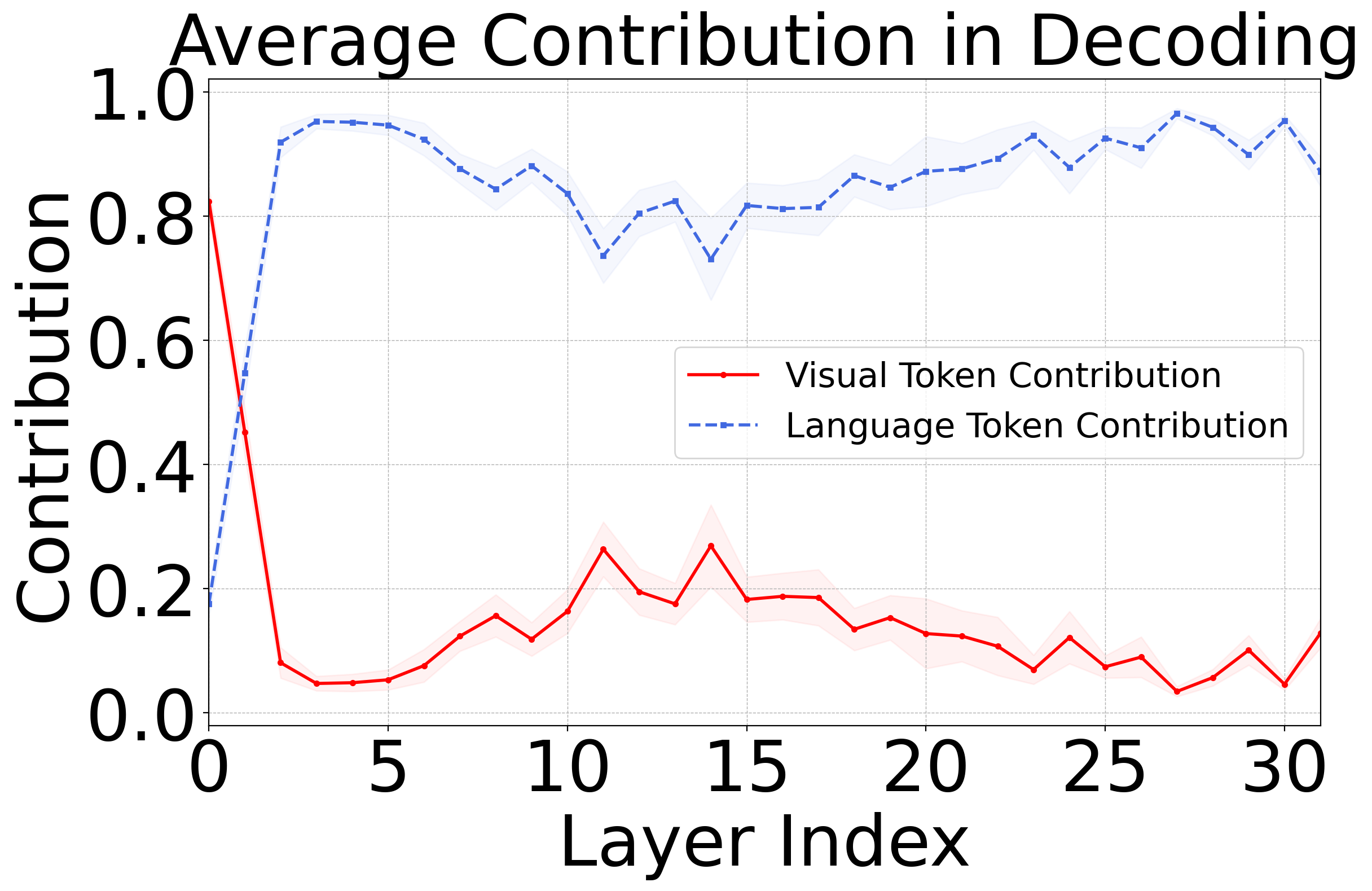
Beyond raw sparsity, the authors quantify how much of a layer’s attention “budget” goes to visual tokens vs. language tokens, using two complementary metrics.
Contribution measures each modality’s share of the filtered (sparsified) attention mass. Let \(T\) be the current sequence length, \(t\) the index of the first decoded token, and \(A^{(l)} \in \mathbb{R}^{T \times T}\) the attention matrix at layer \(l\) for one head:
\[ \text{Contribution}^{(l)}_{mod} := \frac{1}{T - t + 1} \sum_{i \ge t} \frac{\sum_{j \in J_{mod}} \text{ThresholdFilter}(A^{(l)}, p)_{ij}}{\sum_{j \in J_{all}} \text{ThresholdFilter}(A^{(l)}, p)_{ij}} \qquad (3) \]
where \(J_{mod}\) and \(J_{all}\) index one specific modality (vision or language) and all modalities respectively.
Coverage instead measures each modality’s share of the tokens that survive a hard top-k cache-eviction cutoff (rather than share of raw attention mass):
\[ \text{Coverage}^{(l)}_{mod} := \frac{1}{T - t + 1} \sum_{i \ge t} \frac{\sum_{j \in J_{mod}} \text{TopK}(A^{(l)}, k)_{ij}}{\sum_{j \in J_{all}} \text{TopK}(A^{(l)}, k)_{ij}} \qquad (4) \]
\[ \text{TopK}(A, k)_{ij} = \mathbb{1}\!\left[A_{ij} \in \{A_i^{(r-k+1)}, A_i^{(r-k+2)}, \dots, A_i^{(r)}\}\right] \qquad (5) \]
Here \(k := \lfloor \alpha \cdot T \rfloor\), \(r\) is the number of columns of \(A\), and \(A_i^{(n)}\) denotes the \(n\)-th order statistic (rank) of row \(i\) — i.e. \(\text{TopK}\) is an indicator for “this score is among the top-k in its row.”
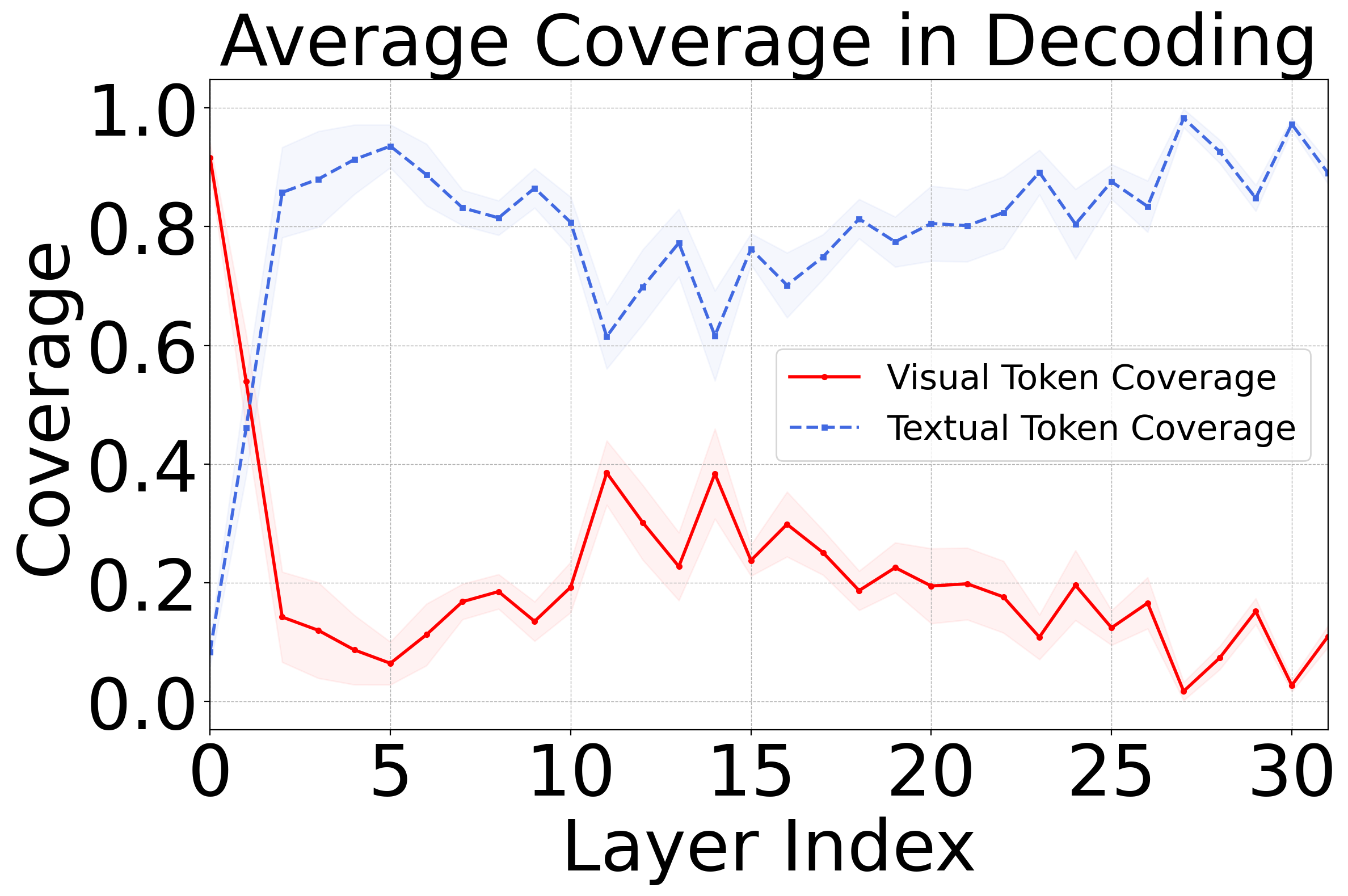
Why this matters for the method: because the vision/language attention split itself varies by layer (heavy vision in layer 1, heavy language from layer 3 onward, with a middle-layer bump in visual importance), the optimal per-layer budget plausibly also depends on the ratio of visual to language tokens in a given prompt. Static, pyramid-style schedules can’t adapt to that; VL-Cache’s per-prompt, per-layer, sparsity-derived allocation can.
Reference glossary of notation
| Symbol | Meaning |
|---|---|
| \(m\) | Number of prompt tokens (visual + language) fed into prefill. |
| \(x_1, \dots, x_m\) | The prompt token sequence. |
| \(k_i^{(l)}, v_i^{(l)}\) | Cached key / value vector for token \(i\) at layer \(l\). |
| \(l, L\) | A transformer layer index; total number of layers. |
| \(h, H\) | An attention-head index; total number of heads. |
| \(d\) | Head dimension. |
| \(A, A^{(l)}\) | Attention score matrix (post-softmax), overall / at layer \(l\). |
| \(A'\) | Post-vision Attention matrix (shorthand used in §4 of the paper). |
| \(p\) | Relative threshold used by ThresholdFilter (set to 1%). |
| \(\gamma^{(l)}, \gamma'^{(l)}\) | Measured sparsity of layer \(l\) — from full attention / from Post-vision Attention. |
| \(\psi\) | A token scoring policy, \(\psi: S \to \mathbb{R}^n\). |
| \(S, S_\psi\) | Indices of cached tokens; indices kept under policy \(\psi\). |
| \(\psi^*, S_{\psi^*}\) | The oracle scoring policy (uses true decoding attention) and its top-k set. |
| \(\tau\) | Number of “post-vision” language tokens (those following the image in the templated prompt). |
| \(\alpha\) | Global target KV cache budget (fraction of tokens to retain). |
| \(\beta^{(l)}\) | Per-layer cache budget fraction produced by Algorithm 1. |
| \(w\) | Fixed window size used by Accumulated Sliding Window Attention (baseline). |
| \(T, t\) | Current total sequence length; index of the first decoded token. |
| \(J_{mod}, J_{all}\) | Index sets for one modality (vision/language) and for all tokens. |
| \(\text{Contribution}^{(l)}_{mod}\) | Modality’s share of filtered attention mass at layer \(l\) (Eq. 3). |
| \(\text{Coverage}^{(l)}_{mod}\) | Modality’s share of surviving (top-k kept) tokens at layer \(l\) (Eq. 4). |
| \(k\) (in TopK) | \(\lfloor \alpha T \rfloor\) — number of tokens retained under a hard top-k cutoff. |
Key takeaways
- VLM attention is not a bigger version of LLM attention: it has a hard modality boundary, and the useful cache-eviction signal concentrates in the language tokens right after the image (“post-vision” tokens), not in the visual tokens themselves or in a generic recency window.
- Attention sparsity varies 70–99% across layers, non-monotonically, and prefill-phase sparsity predicts decoding-phase cache needs (Pearson \(r = 0.695\)) — so budget allocation can be computed once, per-prompt, right after prefill, cheaply.
- VL-Cache = (1) sparsity-derived, per-layer, per-prompt cache budget allocation + (2) Accumulated Post-vision Attention as the token scoring policy — both reuse the same \(O(\tau m)\) Post-vision Attention computation, avoiding the \(O(m^2)\) cost of full attention.
- Empirically: 10% KV cache ≈ full-cache accuracy on Coco-Caption / DocVQA / MathVista across two LLaVA backbones, beating StreamingLLM, H2O, and PyramidKV, especially at aggressive (≤10%) budgets.
- Speed payoff: ≈7× decoding speedup at 128K context, ≈2.3× end-to-end speedup at high batch size, 90% less KV-cache GPU memory, with only 1–6% prefill overhead — the benefit is largest for long-output tasks (captioning, video description, multi-modal chain-of-thought), since end-to-end speedup approaches decoding speedup as output length grows.
Selected references
The following are the works most directly discussed and compared against in this paper (see the paper’s own bibliography for the complete list of ~30 references):
- Xiao et al., Efficient Streaming Language Models with Attention Sinks (StreamingLLM), ICLR 2024 / arXiv:2309.17453.
- Zhang et al., H2O: Heavy-Hitter Oracle for Efficient Generative Inference of Large Language Models, NeurIPS 2023 / arXiv (H2O).
- Zhang et al., PyramidKV: Dynamic KV Cache Compression based on Pyramidal Information Funneling, arXiv:2406.02069.
- Yang et al., PyramidInfer: Pyramid KV Cache Compression for High-Throughput LLM Inference, arXiv:2405.12532.
- He et al., ZipCache: Accurate and Efficient KV Cache Quantization with Salient Token Identification, arXiv:2405.14256.
- Adnan et al., Keyformer: KV Cache Reduction through Key Tokens Selection for Efficient Generative Inference, MLSys 2024.
- Liu et al., KIVI: A Tuning-Free Asymmetric 2-bit Quantization for KV Cache, arXiv:2402.02750.
- Dao, FlashAttention-2: Faster Attention with Better Parallelism and Work Partitioning, arXiv:2307.08691.
- Kwon et al., Efficient Memory Management for Large Language Model Serving with PagedAttention, SOSP 2023.
- Liu et al., Visual Instruction Tuning (LLaVA), NeurIPS 2023, and Improved Baselines with Visual Instruction Tuning (LLaVA-1.6).
- Mathew et al., DocVQA: A Dataset for VQA on Document Images, WACV 2021.
- Lu et al., MathVista: Evaluating Mathematical Reasoning of Foundation Models in Visual Contexts, arXiv:2310.02255.
- Chen et al., Microsoft COCO Captions: Data Collection and Evaluation Server, arXiv:1504.00325.