Source paper: arXiv:2312.12148v1 — submitted 19 December 2023. Index terms: Parameter-efficient, fine-tuning, pretrained language model, large language model, memory usage.
How this document was built. The prose below follows the paper’s own structure and quotes it directly (in quotation marks) wherever a claim is taken verbatim; unquoted text is explanation added for clarity. Figures 1–3 in the original paper are diagrams (an evolution timeline, a taxonomy tree, and three architecture diagrams) — those have been redrawn as Mermaid diagrams here, reconstructed from the paper’s text and captions rather than traced pixel-for-pixel from the original images, so treat them as faithful but not exact reproductions. Figure 4 is a data plot (accuracy-vs-training-step line charts), so it is linked to the original image on arXiv rather than redrawn, per the note in Section 1.10.
Why This Survey Exists
Transformer-based pretrained language models (PLMs) — BERT, RoBERTa, T5, GPT-style models, and now large language models (LLMs) like LLaMA and Falcon — have become the default starting point for almost any NLP task. The standard recipe has always been: pretrain once on a huge unlabeled corpus, then fully fine-tune (update every single parameter) on your downstream task.
That recipe is breaking down under its own weight. The paper opens with a blunt illustration of the problem: model size has exploded from BERT’s 110 million parameters to Falcon’s 180 billion, and “to perform task-specific full fine-tuning with Falcon-180B, a minimum of 5120GB of computational resources may be required.” That’s not a typo — it’s roughly 5 terabytes of GPU memory for one fine-tuning run. Very few labs, let alone individuals, have that kind of hardware.
Parameter-Efficient Fine-Tuning (PEFT) is the family of techniques built to solve exactly this problem. As the authors put it, PEFT “involves employing various deep learning techniques to reduce the number of trainable parameters while still maintaining comparable performance to the full fine-tuning.” Instead of updating all ~100M–100B+ parameters, PEFT methods freeze almost everything and train only a small add-on (sometimes well under 1% of the total parameter count), while trying to match — or in some cases beat — full fine-tuning’s downstream accuracy.
Beyond just saving compute, the paper notes PEFT has a few side benefits worth calling out explicitly:
- Freezing most of the pretrained weights preserves the general knowledge the model learned during pretraining.
- It reduces catastrophic forgetting — the tendency of a fully fine-tuned model to “unlearn” broadly useful capabilities while specializing on a narrow task.
- It mitigates overfitting, which matters a lot when your downstream dataset is small relative to the model’s capacity.
The authors argue that although several PEFT surveys already existed by the time they wrote this one, those surveys had gaps — incomplete taxonomies, missing comparative experiments, or narrow scope. So this paper sets out to do four things comprehensively:
- Propose a clean, five-way taxonomy of PEFT methods: additive, partial, reparameterized, hybrid, and unified fine-tuning.
- Walk through the mechanics of dozens of specific PEFT methods within that taxonomy.
- Run actual experiments with 11 representative PEFT methods across natural language understanding, machine translation, and instruction-tuned generation, measuring both task performance and resource efficiency (parameters + memory).
- Survey PEFT’s use in applications beyond plain task fine-tuning (multi-task learning, cross-lingual transfer, and even backdoor attacks/defenses), and lay out open research directions.
This guide follows that same structure, in the same order, expanding the paper’s dense IEEE-survey prose with analogies, worked-through equations, and comparison tables.
Background: Transformers and Full Fine-Tuning
The Transformer, in the vocabulary PEFT papers use
The Transformer “has emerged as a foundational architecture for numerous PLMs; it adopts an encoder-decoder architecture, comprised of a stack of encoder and decoder layers, each equipped with the self-attention mechanism.” Every PEFT method in this survey inserts itself into, or modifies, one or more of the following pieces:
Step 1 — Project the input into queries, keys, and values. Given an input representation \(X\), three learned linear projections produce:
\[K = XW_k + b_k,\qquad Q = XW_q + b_q,\qquad V = XW_v + b_v\]
Step 2 — Scaled dot-product self-attention. The queries and keys determine how much each token “attends to” every other token, and that attention pattern is used to mix the values:
\[\mathrm{Attn}(Q, K, V) = \mathrm{Softmax}\!\left(\frac{QK^\top}{\sqrt{d}}\right) V\]
Step 3 — Multi-head attention. Rather than doing this once, the model does it \(h\) times in parallel with different learned projections per “head,” then concatenates and projects the result:
\[\mathrm{MHA}(Q, K, V) = \mathrm{Concat}(\mathrm{head}_1, \dots, \mathrm{head}_h) W^O\] \[\mathrm{head}_i = \mathrm{Attn}(QW_i^Q, KW_i^K, VW_i^V)\]
Step 4 — Feed-forward network (FFN). After attention, each position is passed independently through a two-layer MLP with a nonlinearity in between:
\[\mathrm{FFN}(X) = \mathrm{ReLU}(XW_1 + b_1)W_2 + b_2\]
These blocks are wrapped with residual (skip) connections and layer normalization. Keep this picture in mind — attention block, FFN block, residual connections, layer norm — because almost every PEFT method in this survey can be located on it: adapters are new little modules squeezed in after attention and/or FFN; prefix-tuning modifies the \(K\)/\(V\) that attention consumes; LoRA modifies the weight matrices (\(W_q\), \(W_k\), \(W_v\), \(W_1\), \(W_2\), …) themselves via a low-rank side-path; bias-tuning modifies only the \(b\) terms; and so on.
Full fine-tuning: the expensive baseline
“Full fine-tuning of transformer-based PLMs involves training the entire model, including all layers and parameters, on a specific downstream task using task-specific data.” Concretely: you initialize from the pretrained weights, then run ordinary backpropagation and gradient descent on your labeled downstream dataset, updating every weight in the network.
Two problems, both already mentioned above but worth stating plainly here because the rest of the paper is essentially a 20-page answer to them:
- Resource cost. Full fine-tuning “necessitates substantial computational resources and labeled data” — you need to store gradients and optimizer states (e.g., Adam’s two moment buffers) for every parameter, which for a modern LLM multiplies the raw parameter count’s memory footprint several times over.
- Overfitting risk. Full fine-tuning “may give rise to overfitting when the task-specific dataset is small,” since you’re letting a massive number of degrees of freedom adapt to what might be a comparatively tiny labeled set.
PEFT is the response: freeze (almost) everything, train a small, cleverly-placed subset or add-on, and hope to recover most or all of full fine-tuning’s accuracy at a fraction of the cost.
The PEFT Taxonomy
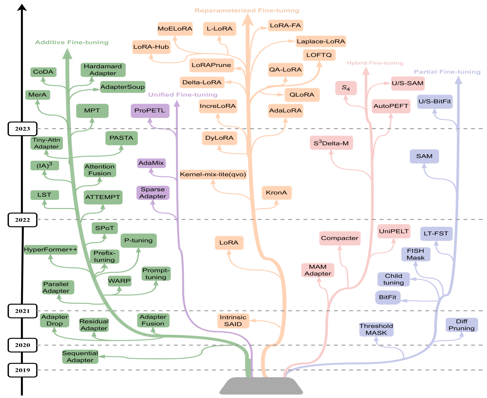
Figure 2 in the paper lays out the taxonomy this whole survey is organized around. It groups every PEFT method into one of five families, based on how the method achieves parameter efficiency:
| Family | Core idea | Where the new/trainable parameters live |
|---|---|---|
| Additive | Freeze the pretrained model, add new trainable modules or tokens | New adapter layers, new soft prompt tokens, new scaling vectors |
| Partial | Freeze most of the model, but unfreeze a subset of existing parameters | A slice of the original weights/biases (e.g. only biases, or a sparse mask over weights) |
| Reparameterized | Represent the weight update \(\Delta W\) in a low-rank / low-dimensional form during training, then merge it back into the full-rank weight | Small low-rank factor matrices (e.g. LoRA’s \(A\), \(B\)) |
| Hybrid | Combine two or more of the above families, either by hand-design or by an automated search | Whatever combination of the above the search/design settles on |
| Unified | Provide a single general framework that different specific PEFT configurations are instances of | A shared architecture/parameterization with per-task or per-layer specialization |
Below is a Mermaid reconstruction of Figure 2’s taxonomy tree — the full method-level detail is reconstructed from the paper’s text and its figure caption, not traced from the source image.
flowchart TD
    PEFT["Parameter-Efficient<br/>Fine-Tuning"] --> ADD[Additive Fine-tuning]
    PEFT --> PART[Partial Fine-tuning]
    PEFT --> REP[Reparameterized Fine-tuning]
    PEFT --> HYB[Hybrid Fine-tuning]
    PEFT --> UNI[Unified Fine-tuning]

    ADD --> ADD1[Adapter-based]
    ADD --> ADD2[Soft Prompt-based]
    ADD --> ADD3[Others]
    ADD1 --> ADD1a["Sequential Adapter, Residual/Parallel<br/>Adapter, CoDA, AdapterDrop, Tiny-Attn,<br/>AdapterFusion, MerA, Hyperformer++, AdapterSoup"]
    ADD2 --> ADD2a["WARP, Prompt-tuning, Prefix-tuning,<br/>P-tuning, SPoT, ATTEMPT, MPT"]
    ADD3 --> ADD3a["(IA)3, LST, PASTA,<br/>AttentionFusion, Hadamard Adapter"]

    PART --> PART1[Bias Update]
    PART --> PART2[Pretrained Weight Masking]
    PART --> PART3[Delta Weight Masking]
    PART1 --> PART1a["BitFit, U/S-BitFit"]
    PART2 --> PART2a["Threshold-Mask, FISH Mask"]
    PART3 --> PART3a["LT-SFT, Child-Tuning,<br/>Diff Pruning, SAM"]

    REP --> REP1[Low-rank Decomposition]
    REP --> REP2[LoRA Derivatives]
    REP1 --> REP1a["Intrinsic SAID, LoRA, KronA"]
    REP2 --> REP2a[Low-rank Adjustment]
    REP2 --> REP2b["LoRA-guided Pretrained<br/>Weight Update"]
    REP2 --> REP2c[Quantization Adaptation]
    REP2 --> REP2d[LoRA-based Improvements]
    REP2 --> REP2e["LoRA-based Multi-task<br/>Fine-tuning"]
    REP2a --> REP2a1["DyLoRA, AdaLoRA, IncreLoRA"]
    REP2b --> REP2b1["Delta-LoRA, LoRAPrune"]
    REP2c --> REP2c1["QLoRA, QA-LoRA, LOFTQ"]
    REP2d --> REP2d1["Kernel-mix-lite,<br/>Laplace-LoRA, LoRA-FA"]
    REP2e --> REP2e1["LoRAHub, MoELoRA, L-LoRA"]

    HYB --> HYB1[Manual Combination]
    HYB --> HYB2[Automatic Combination]
    HYB1 --> HYB1a["MAM Adapter, U/S-MAM,<br/>Compacter, UniPELT"]
    HYB2 --> HYB2a["AutoPEFT, S3Delta-M, S4"]

    UNI --> UNIa["AdaMix, SparseAdapter, ProPETL"]
That’s roughly 45 named methods across five families — this survey’s real value is having them all mapped onto one coherent structure instead of scattered across dozens of individual papers. The original figure is also linked here for reference: Figure 2 — Taxonomy (original image).
The Evolution of PEFT Methods
Figure 1 in the paper shows a branching timeline: “the evolutionary development of PEFT methods in recent years… Models on the same branch have some common features. The vertical position of the models shows the timeline of their release dates.” It’s the same five-family taxonomy, but redrawn so you can see when each method appeared within its branch.
flowchart TB
    subgraph Additive["Additive Fine-tuning"]
        direction TB
        A1["Sequential Adapter (2019)"] --> A2["Residual / Parallel Adapter"] --> A3[CoDA] --> A4[AdapterDrop] --> A5["Tiny-Attn Adapter"] --> A6[AdapterFusion] --> A7["Hyperformer++"] --> A8[MerA] --> A9[AdapterSoup]
    end
    subgraph Partial["Partial Fine-tuning"]
        direction TB
        P1[BitFit] --> P2["U/S-BitFit"] --> P3["Threshold-Mask"] --> P4["FISH Mask"] --> P5["LT-SFT"] --> P6["Child-Tuning"] --> P7["Diff Pruning"] --> P8[SAM]
    end
    subgraph Reparam["Reparameterized Fine-tuning"]
        direction TB
        R1["LoRA (2021)"] --> R2[KronA] --> R3[DyLoRA] --> R4[AdaLoRA] --> R5[QLoRA] --> R6["LoRA-FA"] --> R7["IncreLoRA, DeltaLoRA,<br/>LoRAPrune, QA-LoRA, LOFTQ (2023)"]
    end
    subgraph Hybrid["Hybrid Fine-tuning"]
        direction TB
        H1["MAM Adapter"] --> H2[Compacter] --> H3[UniPELT] --> H4[AutoPEFT] --> H5["S3Delta-M, S4"]
    end
    subgraph Unified["Unified Fine-tuning"]
        direction TB
        U1[AdaMix] --> U2[SparseAdapter] --> U3[ProPETL]
    end
Reading top-to-bottom within each branch tells a coherent story: additive methods came first (Sequential Adapter, 2019) and spent the next few years on efficiency and composition; partial methods explored an orthogonal question — the smallest existing subset of weights you can unfreeze; reparameterized methods exploded in 2021–2023, almost entirely driven by LoRA’s popularity, branching into rank-adaptive, quantization-aware, and multi-task variants; and hybrid/unified methods are the most recent branches, appearing once there was enough of a “menu” of earlier techniques that combining or unifying them became the interesting research question.
Original image for reference: Figure 1 — Evolutionary timeline (original image).
Additive Fine-Tuning
Additive methods leave 100% of the pretrained weights frozen and get their trainable parameters entirely from new modules bolted onto the network. The paper splits these into three groups: adapter-based, soft-prompt-based, and a grab-bag “others” category for methods that don’t fit either mold cleanly.
Adapter-based fine-tuning
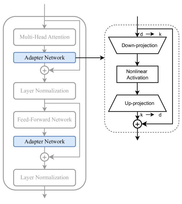
The core idea, introduced by the Sequential Adapter, is to insert a small bottleneck feed-forward module — a down-projection, a nonlinearity, and an up-projection — into each transformer layer, and train only that module (plus, often, layer norm parameters) while freezing everything else. The paper gives the formula for the adapter transformation as a residual bottleneck:
\[X' = \big(\mathrm{ReLU}(X W_{\text{down}})\big) W_{\text{up}} + X\]
where \(W_{\text{down}} \in \mathbb{R}^{d \times k}\) projects the \(d\)-dimensional hidden state down to a small bottleneck dimension \(k \ll d\), and \(W_{\text{up}} \in \mathbb{R}^{k \times d}\) projects it back up. The final \(+X\) is a residual connection, so if the adapter learns to output near-zero, the layer behaves like the untouched pretrained model — a nice property for stable optimization.
Below is a Mermaid reconstruction of Figure 3(a) — the Sequential Adapter’s placement inside a transformer layer, inserted after both the attention and FFN sub-layers, before each residual-add-and-layer-norm step:
flowchart TB
    X["Input X"] --> MHA["Multi-Head Attention"]
    X --> Add1
    MHA --> Add1["+ (residual)"]
    Add1 --> LN1[LayerNorm]
    LN1 --> AD["Adapter: down-proj (d→k) →<br/>nonlinearity → up-proj (k→d)"]
    LN1 --> Add2["+ (residual)"]
    AD --> Add2
    Add2 --> FFN["Feed-Forward Network"]
    Add2 --> Add3["+ (residual)"]
    FFN --> Add3
    Add3 --> LN2[LayerNorm]
    LN2 --> AD2["Adapter: down-proj → nonlinearity → up-proj"]
    LN2 --> Add4["+ (residual)"]
    AD2 --> Add4
    Add4 --> Out[Output]
From that starting point, the paper walks through a lineage of refinements:
- Residual / Parallel Adapter moves the adapter out of the sequential path and runs it in parallel with the attention or FFN sub-layer instead of after it, which reduces the added inference latency since the adapter computation can overlap with the main computation rather than blocking it.
- CoDA (Conditional Adapter) adds a sparse activation mechanism, so only a subset of tokens actually route through the adapter’s extra computation, cutting the added inference cost further.
- AdapterDrop observes that you don’t need adapters in every layer at inference time — you can drop adapters from lower layers dynamically to speed up inference with a small accuracy trade-off.
- Tiny-Attn Adapter adds a small attention module inside the adapter bottleneck itself, letting the adapter capture token-interaction information that a purely position-wise bottleneck MLP would miss.
- AdapterFusion addresses multi-task settings: train separate adapters per task first, then train a small attention-based fusion layer on top that learns how to combine multiple task adapters’ outputs for a new task — a form of non-destructive knowledge composition.
- MerA merges multiple pretrained adapters into a single adapter via parameter averaging/interpolation, rather than keeping and routing between several of them.
- Hyperformer++ uses a shared hypernetwork to generate the adapter weights for each task/layer conditioned on task and layer embeddings, so the number of trainable parameters grows much more slowly as you add more tasks.
- AdapterSoup performs weight averaging (“souping”) across adapters trained on different domains at inference time to improve out-of-domain generalization, without any additional training.
Soft prompt-based fine-tuning
Instead of adding new layers, soft-prompt methods add new trainable tokens (continuous embeddings, not real vocabulary words) that get prepended to the input or to intermediate representations. The model itself stays completely frozen; only these prompt embeddings are trained.
- Prompt-tuning prepends a short sequence of trainable embedding vectors \(P\) directly to the input embeddings, so the model sees \(\hat X = \mathrm{Concat}(P, X)\). Nothing else changes — the frozen transformer just runs forward on this concatenated input. Simplicity is the whole point; the price is that at small model scale, prompt-tuning tends to underperform other PEFT methods notably (this shows up starkly in the paper’s own experiments — see Section 1.10).
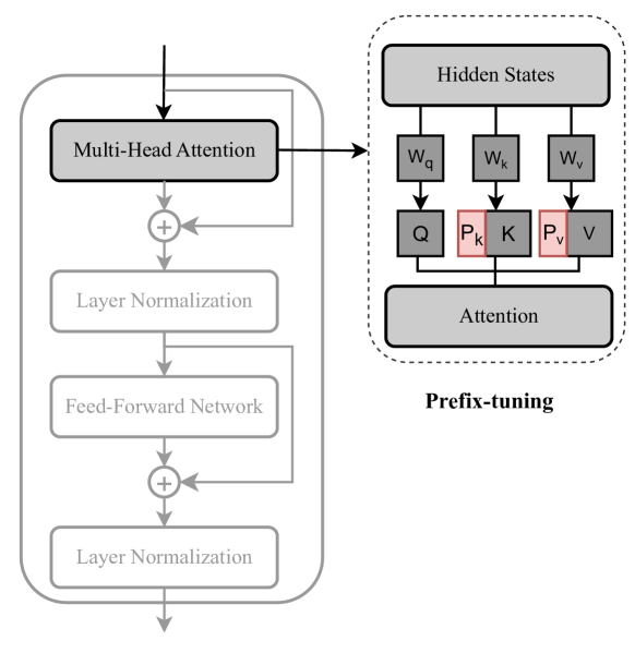
- Prefix-tuning is the more expressive cousin: instead of one prompt inserted at the input layer, it inserts a trainable prefix at every attention layer, directly into the keys and values: \(\mathrm{Attn}(XW_q, [\hat P_k, XW_k], [\hat P_v, XW_v])\). Because it influences every layer’s attention computation rather than just the first layer’s input, prefix-tuning is generally more capable than plain prompt-tuning at a given parameter budget.
Below is a Mermaid reconstruction of Figure 3(b) — where prefix-tuning’s trainable prefixes are concatenated into the attention computation:
flowchart TB
    X["Input X"] --> Q["Q = X W_q"]
    X --> K["K = X W_k"]
    X --> V["V = X W_v"]
    Pk["Trainable Prefix P_k"] --> CatK["Concat(P_k, K)"]
    K --> CatK
    Pv["Trainable Prefix P_v"] --> CatV["Concat(P_v, V)"]
    V --> CatV
    Q --> Attn["Attn(Q, [P_k,K], [P_v,V])"]
    CatK --> Attn
    CatV --> Attn
    X --> Add1["+ (residual)"]
    Attn --> Add1
    Add1 --> LN[LayerNorm]
    LN --> FFN["Feed-Forward Network"]
    Add1 --> Add2["+ (residual)"]
    FFN --> Add2
    Add2 --> Out[Output]
- WARP (“Word-level Adversarial RePrompting”) learns prompt tokens together with a task-specific output/verbalizer layer, framing prompting closer to how masked-language-model prompting is used for classification.
- P-tuning treats the prompt embeddings as free continuous parameters optimized jointly with a small prompt encoder (rather than being tied to actual vocabulary embeddings), improving stability over the naive discrete-prompt-search predecessors it followed.
- SPoT (“Soft Prompt Transfer”) pretrains a soft prompt on one or more source tasks, then uses that as the initialization for a target task’s prompt-tuning, transferring task knowledge purely through the prompt rather than through model weights.
- ATTEMPT extends this transfer idea by learning to attend over and interpolate multiple source-task prompts when initializing/training the target-task prompt, rather than picking just one source.
- MPT (“Multi-task Prompt Tuning”) distills a single shared prompt from a collection of source-task prompts (via a form of low-rank task-shared/task-specific decomposition) and uses that as a strong general starting point across new tasks.
Others
A handful of additive methods don’t fit neatly under “adapter” or “soft prompt”:
- (IA)³ (“Infused Adapter by Inhibiting and Amplifying Inner Activations”) learns a small set of per-channel scaling vectors that element-wise rescale the keys, values, and FFN activations — no bottleneck projections at all, just learned rescaling. It’s strikingly parameter-cheap while remaining competitive on accuracy (see Section 1.10).
- LST (“Ladder Side-Tuning”) trains a small separate “ladder” side network that runs alongside the frozen backbone and reads intermediate activations from it, avoiding backpropagation through the large frozen model entirely — which saves activation memory, not just parameter count.
- PASTA modifies special-token representations (like
[CLS]/[SEP]-style tokens) directly, adding trainable perturbations there instead of throughout the sequence. - AttentionFusion learns to combine multiple existing PEFT modules’ outputs via a trainable attention mechanism over them.
- Hadamard Adapter replaces the usual bottleneck matrix multiplication with an element-wise (Hadamard) product against a trainable vector, an even lighter-weight adapter variant.
Partial Fine-Tuning
Where additive methods add new parameters, partial fine-tuning methods keep the parameter count fixed and instead ask: which existing parameters actually need to move? The rest stay frozen at their pretrained values. The paper splits this family into three groups.
Bias update
- BitFit is the simplest possible partial fine-tuning method: freeze every weight matrix in the network, and train only the bias terms (the \(b\) vectors in \(XW+b\), plus the final classification head). Astonishingly, on many GLUE tasks this recovers most of full fine-tuning’s performance while touching well under 0.1% of the parameters.
- U/S-BitFit extends BitFit with unstructured or structured search over which biases matter most, rather than naively training all of them — a lightweight variant selection step on top of the base idea.
Pretrained weight masking
Rather than restricting which type of parameter to train (bias vs. weight), this group restricts which individual weight entries get updated, via a binary mask \(M\) applied on top of the original weight \(W\):
\[\hat W = M \odot W\]
- Threshold-Mask builds \(M\) by thresholding some importance score per weight, keeping only those above a cutoff \(\tau\): \(M = \mathbb{I}[s_{i,j} > \tau]\).
- FISH Mask uses the Fisher information of each parameter (roughly: how sensitive the loss is to perturbing that parameter) as the importance score, keeping the top-\(k\) most Fisher-important weights: \(M = \mathbb{I}[\text{top-}k(f_{i,j})]\).
Delta weight masking
A closely related but distinct idea: instead of masking the original weight, compute a full gradient-based update \(\Delta W\) as usual, but then mask the update itself before applying it, so only a sparse subset of weights actually change value:
\[\hat W = W + M \odot \Delta W\]
The paper’s Table I in the original catalogs several such methods; reproduced here:
| Method | Weight update | Mask criterion | Mask matrix |
|---|---|---|---|
| Threshold-Mask | \(\hat W = M \odot W\) | Threshold | \(M = \mathbb{I}[s_{i,j} > \tau]\) |
| FISH Mask | \(\hat W = M \odot W\) | Fisher information | \(M = \mathbb{I}[\text{top-}k(f_{i,j})]\) |
| LT-SFT | \(\hat W = W + M \odot \nabla_W \mathcal{L}(W)\) | Absolute difference of parameters | \(M = \mathbb{I}[\text{top-}k(\lvert W_1 - W_0\rvert)]\) |
| Child-Tuning\(_F\) | \(\hat W = W - M \odot \eta\nabla_W \mathcal{L}(W)\) | Bernoulli distribution | \(M \in \{0,1\}^n\) |
| Child-Tuning\(_D\) | \(\hat W = W - M \odot \eta\nabla_W \mathcal{L}(W)\) | Fisher information | \(M = \mathbb{I}[\text{top-}k(f_{i,j})]\) |
| Diff Pruning | \(\hat W = W + M \odot \Delta W\) | Fixed sparsity | \(M \in \{0,1\}^n\) |
| SAM | \(\hat W = W + M\Delta W\) | Analytical solution | \(M_{i,j}=0\ \forall i\neq j;\ M_{i,i}\in\{0,1\}\) |
Reading across the row for Child-Tuning: the “\(F\)” (task-free) variant samples its mask from a simple Bernoulli distribution, essentially randomly deciding which weights are eligible to update each step, while the “\(D\)” (task-driven) variant uses Fisher information like FISH Mask, so it’s a more targeted, task-aware version of the same underlying idea. LT-SFT (“Lottery Ticket Sparse Fine-Tuning”) borrows the lottery-ticket-hypothesis framing: it identifies a sparse “winning” subnetwork of weights (those that moved the most in an initial short fine-tuning run) and restricts the real fine-tuning run to only that subnetwork. Diff Pruning learns a task-specific sparse difference vector under an explicit sparsity budget/regularizer. SAM (Second-order Approximation Method) derives its mask from an analytical, second-order approximation of which weights most reduce the loss, and interestingly restricts updates to the diagonal only — a very tight structural constraint.
Reparameterized Fine-Tuning
This is the family that contains LoRA, almost certainly the single most widely-used PEFT method in practice today, and its many descendants. The core idea: “reparameterized fine-tuning methods utilize low-rank transformation to reduce the number of trainable parameters while allowing operating with high-dimensional matrices.” Rather than training the full weight update \(\Delta W \in \mathbb{R}^{d\times k}\) directly (which has \(d \times k\) trainable numbers), you constrain \(\Delta W\) to be expressible via a much smaller number of parameters, train only those, and reconstruct \(\Delta W\) from them.
Low-rank decomposition
- Intrinsic SAID is the conceptual ancestor here: it’s built on the idea of “intrinsic dimensionality” — the observation that fine-tuning a large model often only needs to move it along a surprisingly low-dimensional subspace of its full parameter space. It reparameterizes the update as \(\Delta W = F(W_r)\), where \(F\) is a (Fastfood) transform projecting a small trainable vector \(W_r \in \mathbb{R}^r\) up into the full parameter space, with \(r \ll d\).
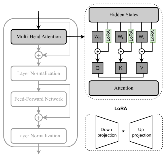
- LoRA (“Low-Rank Adaptation”) makes this idea concrete and practical for transformers specifically: freeze \(W\), and add a trainable update factored as the product of two small matrices,
\[\Delta W = W_{\text{down}} W_{\text{up}}, \qquad W_{\text{down}} \in \mathbb{R}^{d\times r},\ W_{\text{up}} \in \mathbb{R}^{r\times k},\ r \ll \{d,k\}\]
Critically, because \(\Delta W\) is just an ordinary matrix once multiplied out, it can be merged back into \(W\) after training (\(W' = W + \Delta W\)), meaning LoRA adds zero extra inference latency compared to the original model — a major practical advantage over adapters, which do add a small forward-pass cost.
Below is a Mermaid reconstruction of Figure 3(c) — LoRA’s low-rank side-path running parallel to the frozen weight inside the attention block:
flowchart TB
    X["Input X"] --> W["Frozen weight W"]
    X --> Wdown["Trainable A: down-proj (r ≪ d)"]
    Wdown --> Wup["Trainable B: up-proj"]
    W --> Sum["+"]
    Wup --> Sum
    Sum --> MHA["Multi-Head Attention output"]
    X --> Add1["+ (residual)"]
    MHA --> Add1
    Add1 --> LN[LayerNorm]
    LN --> FFN["Feed-Forward Network"]
    Add1 --> Add2["+ (residual)"]
    FFN --> Add2
    Add2 --> Out[Output]
Original image for all three architecture panels: Figure 3 — Sequential Adapter / Prefix-tuning / LoRA architectures (original image).
- KronA replaces the low-rank factorization with a Kronecker product instead: \(\Delta W = W_{\text{down}} \otimes W_{\text{up}}\). Because \(\mathrm{rank}(A\otimes B) = \mathrm{rank}(A)\times\mathrm{rank}(B)\), a Kronecker-product update can represent a higher-rank \(\Delta W\) for the same parameter budget compared to a plain low-rank product — a genuinely different efficiency trade-off than LoRA’s.
LoRA derivatives
LoRA’s simplicity made it extremely easy to extend, and the paper groups the resulting explosion of follow-up work into five sub-categories.
Low-rank adjustment — methods that make the rank \(r\) itself adaptive rather than a fixed hyperparameter:
- DyLoRA trains across a range of ranks \([r_{\min}, r_{\max}]\) simultaneously by randomly truncating the matrices at different ranks \(b\) during training (\(W_{\text{down}\downarrow b} = W_{\text{down}}[:b,:]\), \(W_{\text{up}\downarrow b}=W_{\text{up}}[:, :b]\)), producing a single set of weights that works well across many rank settings so you can pick your accuracy/efficiency trade-off after training without retraining.
- AdaLoRA reparameterizes the update via an SVD-like decomposition, \(\Delta W = P\Lambda Q\) (with \(P,Q\) orthogonal and \(\Lambda\) a diagonal matrix of “singular values”), and then prunes the least important singular values during training — effectively letting each weight matrix in the network get a different, learned, importance-driven rank rather than one fixed rank for everything.
- IncreLoRA grows rank incrementally, formalized as \(\Delta W = W_{\text{down}}\Lambda W_{\text{up}}\) with \(\Lambda = [\lambda_1,\dots,\lambda_r]\) arbitrary constants — starting small and adding rank where it’s needed most as training progresses, the inverse strategy of AdaLoRA’s start-big-and-prune approach.
LoRA-guided pretrained weight update — methods that use the LoRA factors to guide changes to the original frozen weight itself, rather than only adding a separate low-rank path:
- DeltaLoRA periodically folds the change in the low-rank product back into the frozen weight during training: \(W \leftarrow W + \big(W_{\text{down}}^{(t+1)}W_{\text{up}}^{(t+1)} - W_{\text{down}}^{(t)}W_{\text{up}}^{(t)}\big)\), effectively letting the “frozen” weight drift slightly, guided by the LoRA update’s trajectory.
- LoRAPrune combines LoRA with structured pruning, applying a group-wise binary mask on top of the combined weight: \(\delta = (W + W_{\text{down}}W_{\text{up}}) \odot M\), \(M \in \{0,1\}^{1\times G}\), so the model gets smaller (via pruning) and cheaper to fine-tune (via LoRA) at once.
Quantization adaptation — the methods that make LoRA practical at LLM scale by combining it with weight quantization:
- QLoRA quantizes the frozen backbone weights down to 4-bit NormalFloat precision (plus double quantization of the quantization constants themselves, and paged optimizers to handle memory spikes), while still training ordinary full-precision LoRA adapters on top. This is the method responsible for making it feasible to fine-tune a 65B-parameter model on a single consumer/prosumer GPU, and it shows up prominently in this paper’s own memory-efficiency experiments (Section 1.10).
- QA-LoRA uses group-wise quantization, partitioning each weight matrix’s columns into \(L\) groups for finer-grained quantization than QLoRA’s per-tensor approach, and is designed so the final merged model stays quantized after training.
- LOFTQ (“LoRA-Fine-Tuning-aware Quantization”) initializes the LoRA factors specifically to compensate for quantization error, solving \(\Delta W = \mathrm{SVD}(W - Q_t)\) where \(Q_t\) is the quantized weight — instead of quantizing first and hoping LoRA fixes the damage during training, it explicitly initializes LoRA to offset the quantization error from step zero.
LoRA-based improvements — miscellaneous refinements to LoRA’s training dynamics or numerical behavior:
- Kernel-mix-lite treats each attention head as a partially independent estimator, mixing a shared LoRA component (across all heads) with small head-specific components.
- Laplace-LoRA applies a Bayesian Laplace approximation over the LoRA parameters post-training, which the paper’s Further Directions section flags as valuable for improving the calibration of PEFT-tuned models — i.e., making their confidence scores more trustworthy.
- LoRA-FA (“LoRA with Frozen-A”) decomposes the down-projection matrix via QR decomposition and freezes it, updating only the up-projection: \(\Delta W = QRW_{\text{up}}\). Freezing half the LoRA parameters roughly halves LoRA’s already-small memory footprint with little accuracy cost.
LoRA-based multi-task fine-tuning — extending LoRA from single-task to multi-task/transfer settings:
- LoRAHub composes multiple task-specific LoRA modules by learning a weighted combination: \(\hat m = (w_1 W^1_{\text{down}} + \cdots + w_N W^N_{\text{down}})(w_1 W^1_{\text{up}} + \cdots + w_N W^N_{\text{up}})\) — a way to assemble a new-task adapter out of a library of existing task adapters without retraining from scratch.
- MoELoRA combines LoRA with a mixture-of-experts gating mechanism, routing different inputs to different LoRA “experts” based on task-motivated gating signals.
- L-LoRA (“Linearized LoRA”) linearizes the fine-tuned model’s behavior via a first-order Taylor expansion around the pretrained parameters: \(f_{\theta_0}(x;\phi(t)) \approx f_{\theta_0}(x;\phi(0)) + \nabla_\phi f_{\theta_0}(x;\phi(0))^\top(\phi(t)-\phi(0))\), which the paper notes is useful specifically for multi-task model-merging scenarios, since linearized models compose more predictably when you try to add or subtract task vectors from each other.
Table II from the original paper (reproduced in full):
| Method | ΔW reparameterization | Notes |
|---|---|---|
| Intrinsic SAID | \(\Delta W = F(W_r)\) | \(F: \mathbb{R}^r \to \mathbb{R}^d\), \(W_r \in \mathbb{R}^r\) optimized, \(r \ll d\) |
| LoRA | \(\Delta W = W_{\text{down}}W_{\text{up}}\) | \(W_{\text{down}}\in\mathbb{R}^{k\times r}\), \(W_{\text{up}}\in\mathbb{R}^{r\times d}\), \(r\ll\{k,d\}\) |
| KronA | \(\Delta W = W_{\text{down}} \otimes W_{\text{up}}\) | \(\mathrm{rank}(W_{\text{down}}\otimes W_{\text{up}}) = \mathrm{rank}(W_{\text{down}})\times\mathrm{rank}(W_{\text{up}})\) |
| DyLoRA | \(\Delta W = W_{\text{down}\downarrow b}W_{\text{up}\downarrow b}\) | truncated at rank \(b\in\{r_{\min},\dots,r_{\max}\}\) |
| AdaLoRA | \(\Delta W = P\Lambda Q\) | \(PP^\top=P^\top P=I=QQ^\top=Q^\top Q\), \(\Lambda=\mathrm{diag}(\sigma_1,\dots,\sigma_r)\) |
| IncreLoRA | \(\Delta W = W_{\text{down}}\Lambda W_{\text{up}}\) | \(\Lambda=[\lambda_1,\dots,\lambda_r]\), arbitrary constants |
| DeltaLoRA | \(\Delta W = W_{\text{down}}W_{\text{up}}\) | \(W^{(t+1)}\!\leftarrow\! W^{(t)}\!+\!(W^{(t+1)}_{\text{down}}W^{(t+1)}_{\text{up}} - W^{(t)}_{\text{down}}W^{(t)}_{\text{up}})\) |
| LoRAPrune | \(\Delta W = W_{\text{down}}W_{\text{up}}\odot M\) | \(\delta=(W+W_{\text{down}}W_{\text{up}})\odot M\), \(M\in\{0,1\}^{1\times G}\) |
| QLoRA | 4-bit NormalFloat backbone + BF16 LoRA | double-dequantization of quantization constants |
| QA-LoRA | \(\Delta W = W_{\text{down}}W_{\text{up}}\) | \(L\)-group-wise quantization of weight columns |
| LOFTQ | \(\Delta W = \mathrm{SVD}(W - Q_t)\) | \(Q_t = q_N(W - W^{(t-1)}_{\text{down}}W^{(t-1)}_{\text{up}})\), \(q_N\) = \(N\)-bit quantization |
| Kernel-mix-lite | shared + per-head factors | \(B_{\text{LoRA}}\) shared across heads; \(B^h, A^h\) give per-head rank-\(r\) update |
| LoRA-FA | \(\Delta W = QRW_{\text{up}}\) | \(W_{\text{down}}\) frozen (via QR), only \(W_{\text{up}}\) trained |
Hybrid Fine-Tuning
“Hybrid fine-tuning approaches aim to combine various PEFT approaches, such as adapter, prefix-tuning, and LoRA, to leverage the strengths of each method and mitigate their weaknesses.” Instead of picking one family, hybrid methods mix and match. The paper splits hybrid approaches by how the combination is decided: by a human designer, or by an automated search algorithm.
Manual combination
- MAM Adapter (“Mix-And-Match Adapter”) combines a scaled parallel adapter with prefix-tuning, but allocates the budgets asymmetrically: it uses prefix-tuning with a smaller dimension at the attention layers, and gives relatively more trainable parameters to adapters at the FFN layers — a design choice motivated by empirical findings that adapters and prefix-tuning each have a natural “home” (FFN vs. attention) where they’re most effective.
- U-MAM / S-MAM are variants that apply NAS (Neural Architecture Search) together with pruning on top of the MAM Adapter idea, automatically deciding which of the mixed components’ parameters need updating rather than fixing that by hand.
- Compacter builds on the adapter idea but replaces the down/up projection matrices with a parameterized hypercomplex multiplication (PHM) layer, constructing the weight as a sum of Kronecker products: \(W = \sum_i A_i \otimes (s_i t_i^\top)\). This lets Compacter share structure across the projection in a way that needs even fewer trainable parameters than a standard adapter bottleneck.
- UniPELT goes further and incorporates three PEFT types at once — sequential adapter, prefix-tuning, and LoRA — inside a single layer, with a learned gating mechanism that dynamically decides, per input, how much weight to give each submodule’s contribution.
Automatic combination
Rather than a human deciding the mixture recipe, these methods search for it:
- AutoPEFT uses Bayesian optimization to search over an architecture space that includes sequential adapters, parallel adapters, and prefix-tuning, automatically discovering which combination (and where in the network) works best for a given task/budget.
- S³Delta-M performs a differentiable structure search over delta-tuning configurations, combining LoRA, Compacter, BitFit, and LNFit as candidate building blocks across layers, with explicit control over the resulting sparsity.
- S⁴ searches over four axes at once: “layer groupings, trainable parameter allocations, tunable groups, and PEFT module assignments,” dividing the network’s layers into four groups that can each receive a distinct PEFT configuration rather than applying one uniform recipe network-wide.
Unified Fine-Tuning
Unified approaches take a step back from “combine multiple existing methods” and instead try to design one general framework that many specific PEFT configurations fall out of as special cases — providing “a unified framework for fine-tuning, which streamlines the incorporation of diverse fine-tuning methods into a cohesive architecture, ensuring consistency and efficiency.”
- AdaMix treats each adaptation module (e.g., each adapter) as an individual “expert” and uses stochastic routing to select which down-projection/up-projection pairing gets used on a given forward pass, then applies consistency regularization so the multiple experts behave coherently at inference time (where routing is typically averaged rather than stochastic).
- SparseAdapter applies standard network pruning techniques to build a single framework compatible with both adapters and LoRA — it assigns an importance score to each parameter and removes (zeros out) the least important ones past a threshold, unifying pruning-style sparsification with either additive or reparameterized PEFT.
- ProPETL (“Prototype PEFT Learning”) shares a single prototype network across layers and tasks, then uses binary masks to carve out layer-specific and task-specific sub-networks from that one shared prototype — so instead of training separate PEFT parameters per layer or per task from scratch, most of the capacity is shared and only the masks differ. Formally it optimizes \(\max \sum_i \log P(Y_i \mid X_i;\ \theta_{lm}, \theta_{sub})\), where \(\theta_{sub}\) denotes the shared prototype’s sub-network parameters. This method reappears later as one of the paper’s own 11 experimentally-tested PEFT methods (as “ProPELT” — sequential-adapter, prefix, and LoRA variants of the same prototype idea).
Experiments: How Well Do These Methods Actually Work?
Reading about 45 methods in the abstract is one thing; the paper backs it up with real experiments. This is arguably the most practically useful section for a practitioner deciding which PEFT method to reach for.
Setup
The authors picked 11 representative PEFT methods spanning the taxonomy above: sequential adapter (AdapterS), prompt-tuning, prefix-tuning, (IA)³, BitFit, Child-Tuning, LoRA, AdaLoRA, QLoRA, MAM Adapter, and ProPETL. That’s a deliberately broad slice — one or more representatives from additive, partial, reparameterized, and hybrid/unified families each.
They tested across three different model architectures and task types, to check whether findings generalize:
| Model family | Sizes tested | Task | Benchmark |
|---|---|---|---|
| Encoder-only (RoBERTa) | base (125M), large (355M) | Natural Language Understanding | GLUE (“a collection of NLU tasks”) |
| Encoder-decoder (T5) | base (220M), large (770M) | Machine Translation | WMT16 En-Ro (“parallel data pairs”) |
| Decoder-only (LLaMA) | 7B, 13B | Instruction-tuned generation | MMLU, after fine-tuning on Alpaca (“a comprehensive range of 57 disciplines”) |
This is a genuinely useful design choice: it separates PEFT methods that only look good on small encoder models from methods that actually scale to modern decoder-only LLMs.
Fine-tuning performance and parameter efficiency
On RoBERTa/GLUE (Table III in the original): Full fine-tuning (FT) is the 100%-parameter baseline (124.6M params for base, 355.3M for large). Some standout results:
- ProPELT\(_{\text{Adapter}}\) was the strongest performer overall, using only about 1.5% of full fine-tuning’s trainable parameters while exceeding full fine-tuning’s average GLUE score by roughly 1.3 points on RoBERTa-base and 1.65 points on RoBERTa-large — a rare case of a PEFT method clearly beating the full-parameter baseline, not just matching it.
- Prompt-tuning was the weakest performer by a wide margin — despite using the fewest parameters of any method tested (0.61M on base), its average score came in roughly 10 points below full fine-tuning, and it fell apart particularly badly on RTE (a small, hard entailment task): 58.12 vs. full fine-tuning’s 72.20 on RoBERTa-base.
- BitFit, despite only training bias terms, was competitive with — and on RoBERTa-large actually slightly ahead of — several much-more-parameter-hungry methods (88.57 avg vs. AdapterS’s 88.58 avg on RoBERTa-large, at a fraction of the parameter count: 1.32M vs. 19.77M).
- AdapterS (sequential adapter) needed considerably more parameters than most other methods (7.41M on base, 19.77M on large) but delivered correspondingly strong results.
On T5/WMT16 En-Ro (Table IV): (IA)³ was the standout efficiency story — 27.58 BLEU on T5-base with only 0.07M trainable parameters, essentially matching full fine-tuning’s 27.42 BLEU (achieved with 222.9M parameters) using roughly 1/3000th the trainable parameter count. LoRA scored slightly higher still (27.78 BLEU) with 0.88M parameters. On T5-large the gap between all methods and full fine-tuning essentially closed entirely (28.12–28.13 BLEU across FT, (IA)³, and LoRA).
On LLaMA/MMLU (Table VI): Full fine-tuning of LLaMA-7B-Alpaca reached 41.79% 5-shot MMLU accuracy (interestingly, the paper’s Table V shows this number is very sensitive to learning rate: 25.71% at lr=2e-4, 26.65% at lr=5e-5, and 41.79% at lr=1e-6 — a reminder that full fine-tuning at LLM scale needs careful, conservative learning-rate tuning to avoid catastrophic forgetting). Against that baseline:
- LoRA reached 40.67% with 159.9M trainable parameters (2.32% of the model).
- QLoRA reached 39.96% — close to LoRA — while training a comparable number of LoRA parameters (79.9M, since QLoRA’s LoRA adapters are similarly sized) but, crucially, needing far less memory to do it (see below). The paper summarizes: “QLoRA used half the number of trainable parameters of LoRA but achieves comparable performance.”
- (IA)³ was the leanest by far (1.58M params, 0.02% of the model) but paid for it in accuracy — 37.88%, noticeably behind LoRA/QLoRA at this scale.
Figure 4 in the original paper plots 5-shot MMLU accuracy against training steps for each method on both LLaMA-7B and LLaMA-13B (8 subplots total), showing how stable/noisy each method’s accuracy trajectory is during fine-tuning. Because this is a data plot rather than a diagram, it is linked here rather than redrawn:
Memory efficiency
This is where the practical payoff of PEFT becomes unambiguous — Table VII in the original reports peak GPU memory usage across every model and method:
- On RoBERTa-base, full fine-tuning used 5.38GB. Curiously, AdapterS actually used more memory than full fine-tuning here (15.29GB) — inserting adapter modules adds activation memory that, on this small model, ends up outweighing the savings from not storing full-model optimizer states. (IA)³ was the leanest at 2.62GB.
- On LLaMA-7B-Alpaca, the story flips decisively in PEFT’s favor at scale: full fine-tuning required 169.36GB, while QLoRA required only 56.46GB — “QLoRA dramatically reduces GPU memory consumption,” fine-tuning “the LLaMA-7B requiring only 1/3 of the memory required for full fine-tuning.”
- On LLaMA-13B-Alpaca, the effect is even larger: full fine-tuning needed 287.79GB, while QLoRA needed just 66.60GB — “fine-tuning the LLaMA-13B requiring less than 1/4” of full fine-tuning’s memory. Put as relative reductions: “compared with full fine-tuning, IA3, LoRA, and QLoRA reduce memory usage by 33.55%, 39.46%, and 76.86%” respectively at the 13B scale.
The clear headline finding: memory savings from PEFT scale up dramatically with model size. At RoBERTa-base scale, some PEFT methods barely help (or even hurt) memory usage; at LLaMA-13B scale, QLoRA cuts memory requirements by more than 75%. If you’re deciding whether PEFT is “worth it” for your use case, model scale is the single biggest factor.
Applications of PEFT
Beyond plain single-task fine-tuning, the paper surveys three application areas where PEFT’s modularity turns out to be independently useful.
Multi-task learning
“Multi-task learning is a method that involves training a model on multiple related tasks and exploiting the information shared and transferred between them to improve the performance of each task.” PEFT modules are a natural fit here because they’re small, swappable, and composable: “adapters, prompt-tuning, and LoRA utilize additional modules that can be plugged into PLMs and thus can be used for task-specific fine-tuning to improve generalization of multi-task learning.”
Concretely, the survey describes a few recurring strategies: prompt-tuning methods either “utilize pretrained soft prompts from multiple source tasks to initialize the soft prompt of the target task, based on the similarity between the source and target tasks,” or alternatively “employ multi-task data to learn a single shared prompt and transfer it to the target task” (this is exactly the SPoT / MPT idea, applied). Similarly, “a composition of multiple task-specific LoRA modules is also leveraged to transfer knowledge to new tasks” — a nod to LoRAHub. There’s also a more exotic technique using “arithmetic operators, such as the addition and negation operators, to merge parameters of various PEFT methods trained on different tasks” — literally adding or subtracting task-specific PEFT weight deltas as vectors to compose or remove capabilities.
Cross-lingual transfer
“Cross-lingual transfer involves transferring knowledge or models from one language to another. Numerous works have employed PEFT methods, such as adapters, for cross-lingual transfer due to their unique modular design.” Because an adapter is a self-contained, swappable module, you can train language-specific and task-specific adapters separately and combine them at inference time for a language/task pair that was never jointly trained on.
Examples the survey highlights: using “sequential adapter to fine-tune and restore the performance of a multilingual neural machine translation model on high-resource languages,” and using sequential adapters “to transfer a pretrained monolingual model to an unseen language.” The most elaborate example is MAD-X, which employs “language-specific, task-specific, and invertible adapter to learn language-specific and task-specific transformations” — stacking three different adapter types to handle vocabulary mismatches across languages. MAD-G takes this further by generating language adapters on the fly “from language representations based on typological features,” rather than training a fixed adapter per language. There’s also work applying sparse fine-tuning to “train the model on the source language and learn task-specific sparse difference vectors for cross-lingual transfer,” and training “a bilingual language-pair adapter on both the source and target languages for zero-shot cross-lingual transfer.”
Backdoor attacks and defense
This is the section that reframes PEFT’s efficiency as a double-edged sword from a security standpoint. “Backdoor attacks pose a significant security threat, where a small portion of training samples are contaminated with malicious backdoor triggers,” causing a model to “behave normally on benign samples but predict attacker-selected labels on samples containing the predefined triggers.”
The survey notes research going both directions:
- PEFT as an attack vector: researchers have used “PEFT methods to construct backdoor attacks, in which backdoor attacks are directly injected into PEFT modules” — since a PEFT module (like an adapter or LoRA weights) is small, portable, and often distributed/shared independently of the base model (e.g., on model hubs), it’s a plausible vehicle for smuggling a backdoor into a downstream deployment.
- PEFT as a defense: conversely, “PEFT can serve as a backdoor defense solution by reducing the model capacity via optimizing only a small number of parameters” — the idea being that a backdoor typically needs enough free capacity to memorize the trigger-to-target-label mapping, and PEFT’s restricted capacity can make that harder to fit. Related work confirms “PEFT can slightly weaken the backdoor attacks,” while at the same time other work has designed “a novel trojan attack for the PEFT paradigm” specifically — so this is very much an open, actively-contested area rather than a settled one in either direction.
Open Problems and Further Directions
The paper closes its technical content with five concrete directions it thinks the field should pursue next:
- Lightweight hybrid PEFT methods. Existing hybrid methods have mostly combined a narrow set of building blocks — “exploration has been limited to PEFT methods such as adapter, LoRA, prefix-tuning, and BitFit.” The authors want to see hybrid designs that “leverage multiple PEFT methods to improve performance while minimizing the number of trainable parameters,” pointing out that current hybrid approaches typically increase both parameter count and memory usage relative to a single PEFT method, even as they improve accuracy — the efficiency-vs-performance trade-off hasn’t actually been solved by hybridization yet, just shifted.
- More LoRA-derived methods, especially around pruning and quantization. Given how active this sub-area already is, the authors specifically flag “pruning technology and weight quantification” as the most promising directions for further reducing LoRA’s already-small footprint, particularly for LLM-scale deployment.
- Better PEFT tooling/libraries. While libraries like Hugging Face’s
peftand AdapterHub already exist, “not all PEFT methods are currently integrated into these two libraries” — many of the methods cataloged in this survey (especially the newer hybrid/unified ones) don’t yet have accessible, production-ready implementations, which is a real barrier to adoption and fair comparison. - Explainability. Despite the sheer number of PEFT methods proposed, “there is a lack of comprehensive studies exploring the reasons behind their ability to achieve comparable performance and reduce trainable parameters” — i.e., we mostly know PEFT works empirically, but the theoretical why (intrinsic dimensionality arguments aside) is still thin.
- Computer vision and multimodal learning. PEFT research has concentrated almost entirely on NLP; the authors note “there is still significant room for further exploration and exploitation” of PEFT ideas in vision and multimodal (cross-modality) settings, where transformer backbones are now just as dominant as they are in NLP.
Conclusions
The paper’s own summary, paraphrased: this survey delivers a structured, five-category taxonomy (additive, partial, reparameterized, hybrid, unified) covering the PEFT literature, walks through the specific mechanics of dozens of methods within that taxonomy, and backs it up with original experiments across three model architectures (RoBERTa, T5, LLaMA) showing that most PEFT methods achieve “comparable or even better performance compared to full fine-tuning” while using a small fraction of the trainable parameters — and, at LLM scale particularly, dramatically less GPU memory, with quantization-aware methods like QLoRA showing the largest gains. The survey also documents PEFT’s reach beyond single-task fine-tuning into multi-task learning, cross-lingual transfer, and (both offensively and defensively) model security. Looking ahead, the authors frame the central open challenge plainly: “there is a clear need to develop PEFT methods that can effectively reduce computational resource demands and memory usage during fine-tuning” as models keep growing — and position the survey itself as providing “a bird’s-eye view of PEFT methods for PLMs and inspiring further research in this area.”
Quick-Reference Glossary of Every Method Mentioned
| Method | Family | One-line description |
|---|---|---|
| Sequential Adapter | Additive – Adapter | Bottleneck FFN inserted after attention/FFN sub-layers |
| Residual/Parallel Adapter | Additive – Adapter | Adapter runs in parallel with, not after, the sub-layer |
| CoDA | Additive – Adapter | Sparse-activation conditional adapter |
| AdapterDrop | Additive – Adapter | Drops adapters from lower layers at inference |
| Tiny-Attn Adapter | Additive – Adapter | Adds a small attention module inside the bottleneck |
| AdapterFusion | Additive – Adapter | Attention-based fusion of multiple task adapters |
| MerA | Additive – Adapter | Merges adapters via parameter averaging |
| Hyperformer++ | Additive – Adapter | Hypernetwork generates per-task/per-layer adapter weights |
| AdapterSoup | Additive – Adapter | Weight-averages adapters across domains at inference |
| WARP | Additive – Soft Prompt | Prompt tokens + task-specific verbalizer layer |
| Prompt-tuning | Additive – Soft Prompt | Trainable tokens prepended to the input embeddings only |
| Prefix-tuning | Additive – Soft Prompt | Trainable prefixes injected into every layer’s K/V |
| P-tuning | Additive – Soft Prompt | Free continuous prompt embeddings + small encoder |
| SPoT | Additive – Soft Prompt | Transfers a source-task soft prompt as target-task init |
| ATTEMPT | Additive – Soft Prompt | Attends over multiple source-task prompts |
| MPT | Additive – Soft Prompt | Distills one shared prompt from many source-task prompts |
| (IA)³ | Additive – Others | Learned per-channel scaling vectors, no projections |
| LST | Additive – Others | Separate side network avoids backprop through backbone |
| PASTA | Additive – Others | Perturbs special-token representations |
| AttentionFusion | Additive – Others | Attention-based combination of multiple PEFT modules |
| Hadamard Adapter | Additive – Others | Element-wise product adapter, no matrix bottleneck |
| BitFit | Partial – Bias | Trains only bias terms |
| U/S-BitFit | Partial – Bias | Searches which biases matter most |
| Threshold-Mask | Partial – Weight Masking | Masks pretrained weight by importance threshold |
| FISH Mask | Partial – Weight Masking | Masks pretrained weight by Fisher information |
| LT-SFT | Partial – Delta Masking | Lottery-ticket-style sparse update mask |
| Child-Tuning | Partial – Delta Masking | Bernoulli (F) or Fisher-based (D) update mask |
| Diff Pruning | Partial – Delta Masking | Learns sparse difference vector under sparsity budget |
| SAM | Partial – Delta Masking | Analytical, diagonal-only masked update |
| Intrinsic SAID | Reparameterized – Low-rank | Fastfood transform from low-dim intrinsic space |
| LoRA | Reparameterized – Low-rank | Low-rank product \(\Delta W = W_{down}W_{up}\), merges at inference |
| KronA | Reparameterized – Low-rank | Kronecker-product \(\Delta W\) |
| DyLoRA | Reparameterized – LoRA deriv. | Trains across a range of ranks simultaneously |
| AdaLoRA | Reparameterized – LoRA deriv. | SVD-style \(\Delta W\), prunes least-important singular values |
| IncreLoRA | Reparameterized – LoRA deriv. | Incrementally grows rank during training |
| Delta-LoRA | Reparameterized – LoRA deriv. | Folds LoRA’s change back into the frozen weight |
| LoRAPrune | Reparameterized – LoRA deriv. | LoRA + structured pruning mask |
| QLoRA | Reparameterized – LoRA deriv. | 4-bit quantized backbone + full-precision LoRA |
| QA-LoRA | Reparameterized – LoRA deriv. | Group-wise quantization, stays quantized after merge |
| LOFTQ | Reparameterized – LoRA deriv. | LoRA init specifically compensates quantization error |
| Kernel-mix-lite | Reparameterized – LoRA deriv. | Shared + per-attention-head LoRA factors |
| Laplace-LoRA | Reparameterized – LoRA deriv. | Bayesian Laplace approximation for calibration |
| LoRA-FA | Reparameterized – LoRA deriv. | Freezes QR-decomposed down-projection matrix |
| LoRAHub | Reparameterized – LoRA deriv. | Weighted composition of multiple task LoRA modules |
| MoELoRA | Reparameterized – LoRA deriv. | LoRA + mixture-of-experts gating |
| L-LoRA | Reparameterized – LoRA deriv. | First-order Taylor linearization, aids model merging |
| MAM Adapter | Hybrid – Manual | Parallel adapter (FFN) + prefix-tuning (attention) |
| U/S-MAM | Hybrid – Manual | NAS + pruning over MAM Adapter’s components |
| Compacter | Hybrid – Manual | Adapter with hypercomplex-multiplication (Kronecker sum) weights |
| UniPELT | Hybrid – Manual | Adapter + prefix-tuning + LoRA with a learned gate |
| AutoPEFT | Hybrid – Automatic | Bayesian-optimization search over PEFT architecture |
| S³Delta-M | Hybrid – Automatic | Differentiable structure search (LoRA/Compacter/BitFit/LNFit) |
| S⁴ | Hybrid – Automatic | Searches layer grouping + allocation + module assignment |
| AdaMix | Unified | Stochastic routing across adapter “experts” |
| SparseAdapter | Unified | Pruning-based unified framework for adapters/LoRA |
| ProPETL | Unified | Single shared prototype network, masked per layer/task |