This is an explanatory guide, written in my own words, to MobileNetV4: Universal Models for the Mobile Ecosystem [@qin2024mobilenetv4]. It is aimed at someone who wants to understand, reimplement, or apply the ideas, not just skim the abstract.
TL;DR
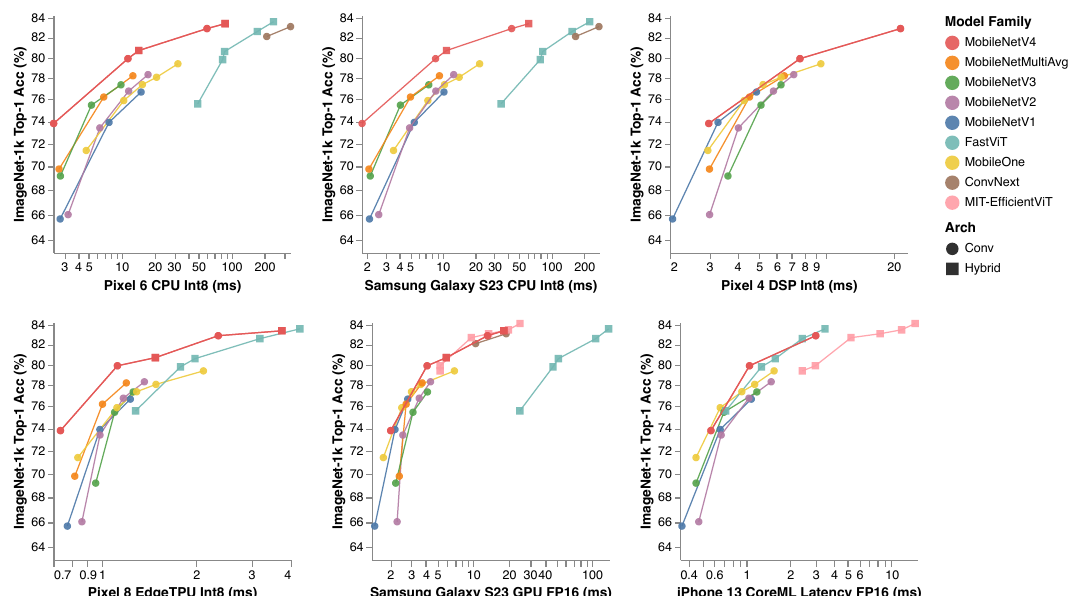
MobileNetV4 (MNv4) is a family of image-classification backbones designed to sit on or near the accuracy/latency Pareto frontier on very different mobile hardware at once: phone CPUs, a Hexagon DSP, mobile GPUs, Apple’s Neural Engine, and Google’s EdgeTPU. The paper’s claim is “mostly Pareto optimal” across these, a deliberately hedged phrase.
Five ingredients produce the result:
- A hardware-independent way to reason about latency: a Roofline model swept over many ridge points, instead of counting MACs.
- Universal Inverted Bottleneck (UIB): an inverted-bottleneck block with two optional depthwise convolutions. One searchable block unifies the classic IB, a ConvNeXt-style block, a ViT-style FFN, and a new “ExtraDW” variant.
- Mobile MQA: multi-query attention with asymmetric spatial downsampling of keys/values, plus an Einsum re-ordering that removes transposes. Reported attention-block speedups are 39% or more on accelerators.
- A refined NAS recipe: a two-stage TuNAS search, trained against an offline JFT-distillation dataset to reduce noise, for 750 epochs.
- A stronger distillation recipe: dynamic dataset mixing plus class-balanced JFT data. With it, MNv4-Hybrid-Large reaches 87.0% ImageNet-1k top-1 (with additional JFT pretraining, see Section 1.9) at 3.8 ms on a Pixel 8 EdgeTPU.
| Model | Top-1 (IN-1k only) | Params (M) | MACs (G) | Distilled top-1 |
|---|---|---|---|---|
| MNv4-Conv-S | 73.8 | 3.8 | 0.2 | 75.5 |
| MNv4-Conv-M | 79.9 | 9.2 | 1.0 | 82.7 |
| MNv4-Hybrid-M | 80.7 | 10.5 | 1.2 | 83.7 |
| MNv4-Conv-L | 82.9 | 31 | 5.9 | 85.9 |
| MNv4-Hybrid-L | 83.4 | 35.9 | 7.2 | 86.6 (87.0 with JFT pretraining) |
- “Universal” means mostly Pareto-optimal on the devices tested, not every device. Hybrid models and ConvNeXt are DSP-incompatible, and hybrids were excluded from the CoreML comparison.
- The 39% MQA speedup is about the attention block’s latency, not the whole network (derivation in Section 1.5).
- Baselines other than MobileNetV1–V3 use their reported accuracies, while MNv4 and the retrained V1–V3 use the new training recipe (see Section 1.11).
Motivation and context
On-device inference is attractive for latency, interactivity, and privacy, because data need not be streamed to a server. The difficulty is that a “mobile” model is deployed on a zoo of chips whose bottlenecks differ. A model hand-tuned for one phone CPU can be poor on an accelerator.
The paper situates itself among four lines of prior work:
- Mobile convnets: MobileNetV1 (depthwise-separable convs), V2 (inverted residuals and linear bottlenecks), GhostNet, MnasNet, MobileOne (re-parameterizable branches) [@howard2017mobilenets; @sandler2018mobilenetv2; @vasu2023mobileone].
- Efficient hybrids (conv + attention): MobileViT, MobileFormer, FastViT, which adds attention only in the last stage [@vasu2023fastvit].
- Efficient attention: linear-complexity approximations (EfficientViT), and downsampling Q/K/V or only K/V (EfficientFormerV2, CMT, NextViT).
- Hardware-aware NAS: NetAdapt, MnasNet, FBNet, MobileNetV3, MobileNet MultiHardware [@howard2019searching; @chu2021multihardware], Once-for-All.
What is new is the combination of a hardware-agnostic analysis tool, one flexible searchable block, an accelerator-friendly attention block, and a better search and distillation recipe.
Hardware-independent efficiency: the Roofline view
Why MACs are not enough
Many papers use MAC count as a latency proxy. That implicitly assumes memory is free. On accelerators, compute capability grows much faster than memory bandwidth, so many layers become memory-bound, and a model with fewer MACs can be slower.
The model
Following the classic Roofline model [@williams2009roofline], each layer \(i\) has a compute time and a memory time, and the slower one determines its latency, because compute and memory overlap roughly in parallel:
\[ \text{ModelTime}=\sum_i \max\big(\text{MACTime}_i,\ \text{MemTime}_i\big),\qquad \text{MACTime}_i=\frac{\text{LayerMACs}_i}{\text{PeakMACs}},\quad \text{MemTime}_i=\frac{\text{WeightBytes}_i+\text{ActivationBytes}_i}{\text{PeakMemBW}} \tag{1}\]
A workload’s operational intensity (OI) is \(\text{LayerMACs}/(\text{WeightBytes}+\text{ActivationBytes})\). A hardware target is summarized by one number, its Ridge Point:
\[ \text{RP}=\frac{\text{PeakMACs}}{\text{PeakMemBW}}\quad[\text{MACs/byte}] \]
A layer whose OI is below the RP is memory-bound on that hardware; above it, compute-bound.
- Counting MACs is the special case RP = 0 (infinite bandwidth, so every \(\text{MemTime}_i=0\)).
- Hardware with the same RP ranks networks the same way, so a sweep of RP from 0 to 500 MACs/byte covers future hardware too, as long as its RP falls in that range.
- Low-RP hardware (CPUs) is mostly compute-bound; high-RP hardware (accelerators) is mostly memory-bound.
The paper’s footnotes add two caveats: the model assumes software implementation does not matter (so tricks with complex memory access, like pruning, look better on paper than on device), and a similar framework was proposed independently by Lavin.
A toy example (Not from the paper)
Let both chips have 3.2 GB/s memory bandwidth, but chip A has 100 GMAC/s (RP ≈ 31, CPU-like) and chip B has 1.39 TMAC/s (RP ≈ 434, accelerator-like). Take two layers: a big conv (200 M MACs, 1 MB traffic, OI = 200) and a final FC layer (1.28 M MACs, about 1.28 MB of weights, OI ≈ 1).
| Layer | Chip A (RP ≈ 31) | Chip B (RP ≈ 434) |
|---|---|---|
| Big conv | MACTime 2.00 ms, MemTime 0.31 ms → 2.00 ms (compute-bound) | MACTime 0.14 ms, MemTime 0.31 ms → 0.31 ms (memory-bound) |
| Final FC | MACTime 0.01 ms, MemTime 0.40 ms → 0.40 ms | MACTime 0.001 ms, MemTime 0.40 ms → 0.40 ms |
The big conv speeds up about 6.5× on the accelerator while the FC layer does not speed up at all and becomes a larger share. This is the mechanism behind the paper’s design logic below.
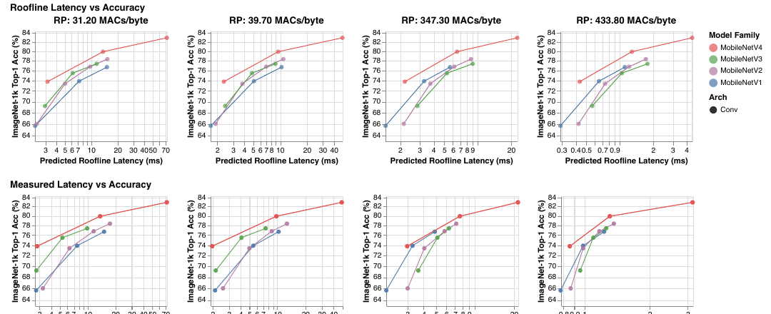
Reading Fig. 2 and Fig. 3
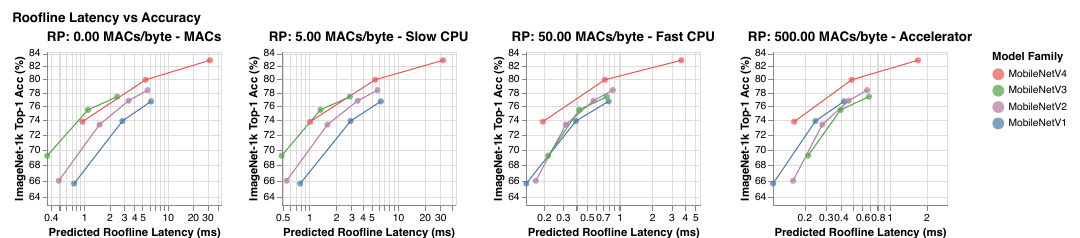
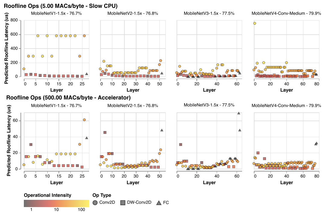
The take-aways are:
- Large Conv2D layers are expensive at low RP but add cheap capacity at high RP.
- FC layers and depthwise convs are cheap at low RP and expensive at high RP.
- MobileNetV1-1.5x and MobileNetV3-Large-1.5x illustrate the two extremes: V3 minimizes MACs at the cost of memory complexity (good on CPUs), V1 spends MACs for capacity (fine on accelerators).
What MNv4’s design takes from this
MNv4 puts expensive, MAC-heavy conv layers at the start of the network (they matter for capacity, and cost only at low RP) and keeps the same large final FC layers in every variant (they matter for accuracy, and cost only at high RP). Because the two costs hurt on opposite hardware classes, no single device pays both at once. The consequence is that smaller variants carry a relatively heavier FC cost on high-RP hardware.
The authors fit a ridge point per device so that the roofline predictions best match measured latency, then compare rank correlation with measured latency against plain MAC counting.
| Execution target | Fitted RP (MACs/B) | \(r_s\) roofline | \(r_s\) MACs |
|---|---|---|---|
| Pixel 6 CPU (Int8) | 31.2 | 0.973 | 0.962 |
| Samsung Galaxy S23 CPU (Int8) | 39.7 | 0.962 | 0.940 |
| Pixel 4 DSP (Int8) | 347.3 | 0.962 | 0.758 |
| Pixel 8 EdgeTPU (Int8) | 433.8 | 0.973 | 0.857 |
The practical reading is that MAC counting is already a decent proxy on CPUs (\(r_s\) of 0.94 to 0.96), but degrades on the DSP and EdgeTPU, where the roofline model stays above 0.96. Note this is a rank correlation across a handful of MobileNet-family models, which says nothing about absolute latency error.
Universal Inverted Bottleneck (UIB)
The idea
The MobileNetV2 inverted bottleneck (IB) is [@sandler2018mobilenetv2]: 1×1 pointwise (PW) expand → depthwise (DW) conv → 1×1 PW project. UIB makes one change: it adds an optional DW before the expansion and makes the middle DW optional too. Two on/off switches give four combinations, and NAS picks per block which to use.
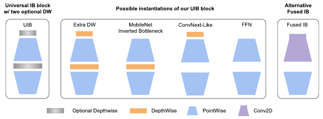
The same figure redrawn as a Mermaid diagram (my redraw of the paper’s figure, with the structure read off the image and from the paper’s architecture tables):
flowchart LR
  subgraph UIB["UIB (general form)"]
    direction TB
    u0([input]) --> u1["DW K1 (optional)"] --> u2["PW expand 1x1"] --> u3["DW K2 (optional)"] --> u4["PW project 1x1"] --> u5([output])
  end
  subgraph EDW["ExtraDW (K1 and K2)"]
    direction TB
    e0([input]) --> e1["DW K1"] --> e2["PW expand"] --> e3["DW K2"] --> e4["PW project"] --> e5([output])
  end
  subgraph IB["MobileNet IB (K2 only)"]
    direction TB
    i0([input]) --> i2["PW expand"] --> i3["DW K2"] --> i4["PW project"] --> i5([output])
  end
  subgraph CNX["ConvNeXt-like (K1 only)"]
    direction TB
    c0([input]) --> c1["DW K1"] --> c2["PW expand"] --> c4["PW project"] --> c5([output])
  end
  subgraph FFN["FFN (neither)"]
    direction TB
    f0([input]) --> f2["PW expand"] --> f4["PW project"] --> f5([output])
  end
  subgraph FIB["Fused IB (alternative)"]
    direction TB
    g0([input]) --> g2["kxk Conv2D expand"] --> g4["PW project 1x1"] --> g5([output])
  end
  UIB --> EDW
  UIB --> IB
  UIB --> CNX
  UIB --> FFN
The four instantiations
| Instantiation | DW before expansion (K1) | DW between (K2) | What it buys you |
|---|---|---|---|
| IB (MobileNetV2) | – | ✓ | Spatial mixing on the expanded (wide) activations: more capacity, higher cost |
| ConvNeXt-like | ✓ | – | Cheaper spatial mixing, so larger kernels are affordable (mixing happens before expansion) |
| ExtraDW (new) | ✓ | ✓ | Cheaply increases depth and receptive field; combines the benefits of ConvNeXt-like and IB |
| FFN | – | – | Two pointwise convs with activation and norm: very accelerator-friendly, but best used alongside other blocks |
The paper notes ExtraDW can be viewed as a MobileNetV1-style factorization of two standard convolutional blocks. At every stage UIB lets the network choose an ad-hoc spatial vs channel mixing trade-off, enlarge the receptive field where needed, and maximize compute utilization.
Why this stays NAS-friendly
The PW expansion and projection weights are shared across the candidate instantiations; only the DW ops are the searchable options. The paper reports that a SuperNet-based search then shares over 95% of the parameters between candidates, so the search space is manageable.
Fused IB
A \(k\times k\) FusedIB replaces the expand-PW + DW pair with a single \(k\times k\) full Conv2D followed by a 1×1 PW [@akin2022edgetpu]. All MNv4 model stems use FusedIBs (Appendix D).
Does UIB help? (Table 1)
| Search space | Top-1 | GMACs | MParams | Pixel 8 EdgeTPU |
|---|---|---|---|---|
| UIB (full) | 83.3% | 6.2 | 33.0 | 2.68 ms |
| ConvNeXt-like only | 83.2% | 6.9 | 35.1 | 2.69 ms |
| IB only | 82.3% | 6.1 | 32.4 | 2.61 ms |
The UIB vs ConvNeXt gap is 0.1 points with lower MACs, and the IB-only search is cheaper in MACs and latency (so not iso-cost). The text I have reports one number per search and no variance, so the +1.0 over IB is the more convincing signal than the +0.1 over ConvNeXt. This is my reading, not a claim by the authors.
Where NAS actually puts each block (Appendix D)
The authors summarize what TuNAS chose in the final Conv models:
- ExtraDW tends to appear at the start of each searchable stage, where resolution drops sharply. The two DWs enlarge the receptive field and soften the resolution loss. It is also common in early stages.
- FFN and ConvNeXt-like blocks show up in the final layers, where earlier layers have already mixed spatially and channel mixing gives more marginal gain.
A PyTorch sketch (Not from the paper)
The paper’s reference implementation is in TensorFlow Model Garden (footnote 1 of the paper); a timm port also exists (footnote 7). The sketch below is my own illustration of the block’s logic, not the official code.
import torch
import torch.nn as nn


def conv_bn(c_in, c_out, k, stride=1, groups=1, act=True):
    layers = [
        nn.Conv2d(c_in, c_out, k, stride, padding=k // 2, groups=groups, bias=False),
        nn.BatchNorm2d(c_out),
    ]
    if act:
        layers.append(nn.ReLU(inplace=True))  # paper favours ReLU/BN (hardware support)
    return nn.Sequential(*layers)


class UIB(nn.Module):
    """Universal Inverted Bottleneck.
    start_dw_k: kernel of the optional DW *before* expansion (0 = absent)
    mid_dw_k:   kernel of the optional DW *between* expand and project (0 = absent)
      (0, 3|5) -> IB          (3|5, 0) -> ConvNeXt-like
      (k1, k2) -> ExtraDW     (0, 0)   -> FFN
    """

    def __init__(self, c_in, c_out, expand_ratio=4, start_dw_k=0, mid_dw_k=3, stride=1):
        super().__init__()
        c_mid = int(round(c_in * expand_ratio))
        self.use_res = stride == 1 and c_in == c_out  # assumption: standard IB-style residual
        # Where the stride goes is NOT specified in the paper text: verify against the
        # official TF code / timm before comparing against published latencies.
        s_start = stride if (start_dw_k and not mid_dw_k) else 1
        s_mid = stride if mid_dw_k else 1
        if stride > 1 and not (start_dw_k or mid_dw_k):
            raise ValueError("an FFN-type UIB cannot downsample")
        self.start_dw = conv_bn(c_in, c_in, start_dw_k, s_start, groups=c_in, act=False) if start_dw_k else nn.Identity()
        self.expand = conv_bn(c_in, c_mid, 1)
        self.mid_dw = conv_bn(c_mid, c_mid, mid_dw_k, s_mid, groups=c_mid) if mid_dw_k else nn.Identity()
        self.project = conv_bn(c_mid, c_out, 1, act=False)

    def forward(self, x):
        y = self.project(self.mid_dw(self.expand(self.start_dw(x))))
        return x + y if self.use_res else y


class FusedIB(nn.Module):
    """k x k full conv (expand) -> 1x1 project; used in MNv4 stems."""

    def __init__(self, c_in, c_out, expand_ratio=4, k=3, stride=1):
        super().__init__()
        c_mid = int(round(c_in * expand_ratio))
        self.conv = conv_bn(c_in, c_mid, k, stride)
        self.project = conv_bn(c_mid, c_out, 1, act=False)
        self.use_res = stride == 1 and c_in == c_out

    def forward(self, x):
        y = self.project(self.conv(x))
return x + y if self.use_res else yAppendix D lists each model block by block: input resolution and channels, block type, K1/K2 kernels, expanded dimension, output dimension, and stride. A faithful reimplementation is mostly a loop over those rows, calling the block with expand_ratio = expanded_dim / in_channels. Note the expansion ratios vary between blocks (for example 2, 4, and 6 in MNv4-Conv-M), which matters for the NAS discussion in Section 1.6.2.
Mobile MQA
Background: MHSA vs MQA
Multi-head self-attention (MHSA) projects queries, keys, and values separately per head. Multi-query attention (MQA) [@shazeer2019mqa] keeps multiple query heads but shares a single key head and a single value head across all of them. The paper cites language-model work showing that sharing one key/value head does not noticeably cost accuracy.
Why MQA suits mobile vision
The argument is again about operational intensity. When the number of tokens is small relative to the feature dimension, loading separate K/V projections per head is mostly memory traffic. Sharing them reduces bandwidth and raises operational intensity. In mobile hybrids this regime is typical, because attention is used only in the low-resolution, high-channel final stages and batch size is usually 1. To the authors’ knowledge this is the first use of MQA for mobile vision.
Asymmetric spatial downsampling
Borrowing the “asymmetric” spirit of MQA, they add spatial reduction attention (SRA, from Pyramid Vision Transformer [@wang2021pvt]) so keys and values live at lower resolution than queries. Two differences from PVT: the downsampling is a stride-2 3×3 depthwise conv instead of average pooling, which is cheap and adds capacity. The justification is that neighbouring tokens in hybrid models are already correlated thanks to early spatial-mixing convs.
The resulting block (the paper’s Eq. 2):
\[ \text{MobileMQA}(X)=\text{Concat}(\text{attn}_1,\dots,\text{attn}_n)\,W^O,\qquad \text{attn}_j=\text{softmax}\!\left(\frac{(XW^{Q}_j)\,(\text{SR}(X)W^{K})^{\top}}{\sqrt{d_k}}\right)\text{SR}(X)W^{V} \tag{2}\]
Here \(\text{SR}\) is the stride-2 DW conv when spatial reduction is used, or the identity otherwise. Note \(W^K\) and \(W^V\) carry no head index (the sharing), while \(W^Q_j\) does.
The measured gains
| Model (MNv4-Conv-L base, 3 attention blocks in last stage) | Top-1 | MACs (G) | Params (M) | Pixel 7 EdgeTPU | Pixel 8 EdgeTPU | S23 GPU |
|---|---|---|---|---|---|---|
| base | 84.88 | 6.0 | 30.9 | 4.31 ms | 2.35 ms | 13.15 ms |
| + 3 MHSA | 85.27 | 6.7 | 36.0 | 9.69 ms | 2.76 ms | 16.46 ms |
| + 3 MQA | 85.24 | 6.5 | 34.7 | 5.16 ms | 2.60 ms | 15.10 ms |
| relative to MHSA | −0.03 | −28.6% | −25.5% | −84.2% | −39.0% | −41.1% |
The relative-improvement row considers only the latency added by the attention blocks, not the whole model. I checked the arithmetic from the table: on Pixel 8, MHSA adds 2.76 − 2.35 = 0.41 ms and MQA adds 2.60 − 2.35 = 0.25 ms, which is −39.0%. On Pixel 7 the added latency drops from 5.38 ms to 0.85 ms (−84.2%). Whole-model latency improves much less (for example 9.69 → 5.16 ms on Pixel 7). MACs and params percentages likewise refer to the added increments (0.7 → 0.5 G MACs; 5.1 → 3.8 M params).
| Downsampling of K/V (Hybrid-M, S23) | Top-1 | MACs (G) | CPU (ms) | GPU (ms) |
|---|---|---|---|---|
| No | 80.77 | 1.285 | 15.8 | 7.4 |
| Yes (stride-2) | 80.71 | 1.245 | 12.8 | 5.9 |
| Gain | −0.06 | +3% | +23% | +25% |
The Einsum optimization (Appendix G)
Even plain MQA, though faster than MHSA, was still about 12× slower than UIB for the same MACs. The culprit was not arithmetic but transposes: on-device, an Einsum is lowered to transposes, reshapes, and batched matmuls. Transposes cost zero MACs but need a full read and write of the tensor, so they are pure memory traffic.
Two rules explain when transposes appear:
- Contracted and non-contracted indices are not contiguous in an input. A matmul needs the contracted indices adjacent so that reshaping to 2-D is free.
- Interleaved non-contracted indices or a reordered output: the output indices must come out in an order that avoids a post-matmul transpose.
The fix is only a re-ordering of indices in the Einsum strings and in the weight tensor layout:
# Slow: 2 transposes (non-contracted h, k interleaved with n; output reordered)
Q = tf.einsum("bnd,hdk->bhnk", X, P_q)
# Fast: no transpose
Q = tf.einsum("bnd,dhk->bnhk", X, P_q)

# Slow: 2 transposes (contracting h,v are not adjacent in the operands)
Y = tf.einsum("bhnv,hdv->bnd", O, P_o)
# Fast: no transpose
Y = tf.einsum("bnhv,hvd->bnd", O, P_o)
(Fig. 11 of the paper writes the optimized output projection as "bnhv,dhv->bnd", with the weight stored as dhv. That is the same idea as the hvd form in the Appendix G text: the contracted axes h, v are adjacent in both operands, so no transpose is needed. Treat the weight-axis order as a layout choice, not a fixed rule.)
| Variant (MNv4-Conv-L + 3 attention blocks) | Pixel 7 EdgeTPU | Pixel 8 EdgeTPU |
|---|---|---|
| base model | 4.31 ms | 2.35 ms |
| MQA, vanilla Einsum | 7.00 ms | 2.64 ms |
| Mobile MQA, optimized Einsum | 5.16 ms | 2.60 ms |
| Improvement on added latency | −68.4% | −13.8% |
The authors also report almost a 3× training speed-up with tf.keras on Google Tensor v4, so the benefit is not specific to inference.
When porting attention to an accelerator, profile the op graph, not the FLOP count. Layout (the order of axes) can dominate. This is the same operational-intensity story as Section 1.3, expressed at the tensor-layout level.
A PyTorch sketch (Not from the paper)
The paper states that at the time of writing there was no PyTorch implementation of Mobile MQA, which is why hybrids were left out of the CoreML comparison. The following is my own sketch of the math in Equation 2; it does not reproduce the TensorFlow layout optimization, and PyTorch/CoreML lowering will differ.
import torch
import torch.nn as nn


class MobileMQA(nn.Module):
    """Multi-query attention on a (B, C, H, W) feature map, with optional stride-2 DW
    spatial reduction applied to keys/values only (sketch of Eq. 2)."""

    def __init__(self, dim, num_heads=4, key_dim=64, value_dim=64, kv_downsample=True):
        super().__init__()
        self.h, self.kd, self.vd = num_heads, key_dim, value_dim
        self.q = nn.Conv2d(dim, num_heads * key_dim, 1, bias=False)   # per-head queries
        self.sr = (
            nn.Sequential(
                nn.Conv2d(dim, dim, 3, stride=2, padding=1, groups=dim, bias=False),
                nn.BatchNorm2d(dim),
            )
            if kv_downsample
            else nn.Identity()
        )
        self.k = nn.Conv2d(dim, key_dim, 1, bias=False)    # ONE shared key head
        self.v = nn.Conv2d(dim, value_dim, 1, bias=False)  # ONE shared value head
        self.o = nn.Conv2d(num_heads * value_dim, dim, 1, bias=False)

    def forward(self, x):
        B, _, H, W = x.shape
        N = H * W
        q = self.q(x).view(B, self.h, self.kd, N).transpose(2, 3)   # B,h,N,kd
        src = self.sr(x)
        k = self.k(src).flatten(2)                                   # B,kd,M
        v = self.v(src).flatten(2).transpose(1, 2)                   # B,M,vd
        attn = (q @ k.unsqueeze(1)) * self.kd ** -0.5                # B,h,N,M
        attn = attn.softmax(dim=-1)
        out = attn @ v.unsqueeze(1)                                  # B,h,N,vd
        out = out.transpose(1, 2).reshape(B, N, self.h * self.vd)    # B,N,h*vd
        out = out.transpose(1, 2).reshape(B, self.h * self.vd, H, W)
        return self.o(out)
Designing the models
Design philosophy: simplicity
Before searching, the authors ran correlation analyses between cost models and hardware, and kept only components whose costs correlate well across devices and that sit near the Pareto frontier. Findings that shaped the search space:
- Multi-path blocks (group convs, ShuffleNet-style) have low MACs but are inefficient because of memory-access complexity.
- Modules with weak hardware support: Squeeze-and-Excite, GELU, and LayerNorm are poorly supported on DSPs (LayerNorm lags BatchNorm), and SE is slow on accelerators.
- Conventional components win: depthwise and pointwise convs, ReLU, BatchNorm, and plain attention.
From these they derived three principles: use standard widely supported components, use flexible UIB blocks, and use straightforward attention (Mobile MQA).
Neural architecture search
NAS uses TuNAS [@bender2020tunas] with modifications, and a separate search per model size (rather than EfficientNet-style fixed scaling rules [@tan2019efficientnet]).
Two-stage search
TuNAS with weight sharing tends to be biased toward smaller filters and expansion factors, partly because the UIB depthwise layers differ in parameter count from other options. The remedy is to separate coarse and fine decisions:
flowchart TD
  A["Stage 1: coarse-grained search<br/>fixed block: IB, expansion 4, 3x3 DW<br/>search 'filter sizes'"] --> B["Stage 2: fine-grained search<br/>per block: presence of 2 DWs (K1, K2)<br/>kernel 3x3 or 5x5 each<br/>expansion held at 4"]
  B --> C["Final UIB macro-architecture<br/>(MNv4-Conv-S/M/L)"]
  D["Offline JFT-distillation dataset<br/>(reduces reward noise)"] -.-> A
  D -.-> B
| Search | Top-1 (val) | Top-1 (train) | Pixel 6 EdgeTPU |
|---|---|---|---|
| One-stage | 81.26 | 74.64 | 3.85 ms |
| Two-stage | 81.48 (+0.22) | 78.24 (+3.60) | 3.67 ms (−4.68%) |
The paper says the coarse stage determines “filter sizes” while the block is fixed at expansion 4 with a 3×3 kernel. Since the kernel is fixed, “filter sizes” most plausibly means channel widths, not kernel sizes. This is my interpretation [Likely], not stated in the text.
Also, stage 2 is described as holding the expansion factor at 4, yet the final architectures in Appendix D contain other expansion ratios (for example, 80→160 is ×2 and 80→480 is ×6 in MNv4-Conv-M). So the expansion factor must be searched or set elsewhere; the text as extracted does not say where.
Training the supernet on distilled data
TuNAS’s reward needs an accurate architecture-quality signal, but ImageNet-1k training is sensitive to augmentation, regularization, and hyperparameters, and a changing set of sampled architectures makes a stable recipe hard. The fix is an offline distillation dataset (the JFT-based dataset of Section 1.9) as the search training set. They also train the search for 750 epochs, citing evidence [@bello2021revisiting] that depth-scaling beats width-scaling under long training, which yields deeper models.
| NAS training data | Top-1 (val/train) | MACs | Params | Pixel 4 GPU | Pixel 6 CPU |
|---|---|---|---|---|---|
| ImageNet-1k | 82.4 / 72.9 | 7.2G | 43.5M | 59.2 ms | 70.4 ms |
| JFT distillation | 82.3 / 74.0 | 6.2G | 34.4M | 51.0 ms | 67.3 ms |
| Gain | −0.1 / +1.1 | +13.9% | +20.9% | +13.9% | +4.4% |
Search space and targets (Appendix A)
- Fixed initial layers: a 3×3 stride-2 Conv2D, then a NAS-optimized stride-2 FusedIB stage.
- Searched: the number of UIB blocks and each block’s instantiation for the remaining four stages.
- Fixed head: same as MobileNetV3.
- Pointwise convs have low operational intensity at high resolution, so MAC-dense ops were favoured in the early layers.
| Model | Search target |
|---|---|
| MNv4-Conv-S | 285 M MACs and 0.2 ms (Pixel 6 EdgeTPU, 224 px) |
| MNv4-Conv-M | 0.6 ms (Pixel 6 EdgeTPU, 256 px) |
| MNv4-Conv-L | 2.3 ms (Pixel 6 EdgeTPU) and 2.0 ms (Pixel 7 EdgeTPU), 384 px |
Key claim: because the space is restricted to components with well-correlated cost models, optimizing EdgeTPU latency alone produced universally efficient models. This is why a single search target suffices, and it is also the biggest assumption to test if you adapt the recipe to other hardware.
From Conv to Hybrid models
Attention is most effective in the last stages, in line with other hybrids. MNv4-Hybrid models interleave Mobile MQA blocks with UIB blocks in the late stages. The architecture tables show the pattern: in Hybrid-M, MQA blocks alternate with ExtraDW/ConvNeXt/FFN blocks at the 16×16 stage and again at 8×8.
The MNv4 model family
Five models: Conv-S, Conv-M, Conv-L (pure convolutional, built from UIB blocks) and Hybrid-M, Hybrid-L (Conv blocks interleaved with Mobile MQA). All use a FusedIB stem and the MobileNetV3-style head (1×1 conv to 960, global average pool, 1×1 conv to 1280, 1×1 classifier to 1000).
| Model | Input res. | Notes from the paper’s tables |
|---|---|---|
| Conv-S | 224 | Smallest; 3.8 M params; ExtraDW at stage starts, IB blocks in the middle |
| Conv-M | 256 | Mostly ExtraDW, with ConvNeXt-like and FFN blocks sprinkled in |
| Hybrid-M | 256 | Conv-M-like backbone with Mobile-MQA blocks interleaved at the 16×16 and 8×8 stages |
| Conv-L | 384 | 24 → 512 channels, longest ExtraDW/ConvNeXt stacks |
| Hybrid-L | 384 | Conv-L-like backbone with Mobile-MQA interleaved at the 24×24 and 12×12 stages |
| Input | Block | DW K1 | DW K2 | Expanded | Output | Stride |
|---|---|---|---|---|---|---|
| 224²×3 | Conv2D | – | 3×3 | – | 32 | 2 |
| 112²×32 | FusedIB | – | 3×3 | 32 | 32 | 2 |
| 56²×32 | FusedIB | – | 3×3 | 96 | 64 | 2 |
| 28²×64 | ExtraDW | 5×5 | 5×5 | 192 | 96 | 2 |
| 14²×96 | IB (×4) | – | 3×3 | 192 | 96 | 1 |
| 14²×96 | ConvNeXt | 3×3 | – | 384 | 96 | 1 |
| 14²×96 | ExtraDW | 3×3 | 3×3 | 576 | 128 | 2 |
| 7²×128 | ExtraDW | 5×5 | 5×5 | 512 | 128 | 1 |
| 7²×128 | IB | – | 5×5 | 512 | 128 | 1 |
| 7²×128 | IB | – | 5×5 | 384 | 128 | 1 |
| 7²×128 | IB (×2) | – | 3×3 | 512 | 128 | 1 |
| 7²×128 | Conv2D | – | 1×1 | – | 960 | 1 |
| 7²×960 | AvgPool | – | 7×7 | – | 960 | 1 |
| 1²×960 | Conv2D | – | 1×1 | – | 1280 | 1 |
| 1²×1280 | Conv2D | – | 1×1 | – | 1000 | 1 |
Results
ImageNet-1k classification
Protocol. MNv4 models are trained on the ImageNet-1k training split only (no extra data) and evaluated on its validation split. MobileNetV1–V3 were retrained with modern recipes (+3.4 to 74.0 for V1, +1.4 to 73.4 for V2, +0.3 to 75.5 for V3) so the comparison isolates architecture. Other baselines (MobileOne, FastViT, EfficientViT, ConvNeXt, NextViT) use their reported accuracies with the authors’ own latency measurements.
| Model | Top-1 | Params (M) | MACs (G) | P6 CPU | P8 EdgeTPU | iPhone 13 CoreML | P4 Hexagon | P7 GPU | S23 CPU | S23 GPU |
|---|---|---|---|---|---|---|---|---|---|---|
| MobileNet-V3L-0.5x | 69.2 | 2.7 | 0.1 | 2.4 | 0.8 | 0.45 | 3.5 | 9.9 | 2.0 | 2.1 |
| MobileNet-V2 | 73.4 | 3.5 | 0.3 | 5.0 | 0.7 | 0.7 | 3.9 | 13.6 | 4.1 | 2.5 |
| MNv4-Conv-S | 73.8 | 3.8 | 0.2 | 2.4 | 0.7 | 0.6 | 2.4 | 8.4 | 1.8 | 2.0 |
| MobileNet-V1 | 74.0 | 4.2 | 0.6 | 6.1 | 0.8 | 0.7 | 3.2 | 13.0 | 4.6 | 2.1 |
| MobileOne-S4 | 79.4 | 14.8 | 1.5 | 26.7 | 1.7 | 1.5 | 9.0 | 28.6 | 19.4 | 5.9 |
| FastViT-S12 | 79.8 | 8.8 | 1.8 | 83.0 | 1.8 | 1.6 | Failed | 75.0 | 69.2 | 47.0 |
| MIT-EfficientViT-B1-r224 | 79.4 | 9.1 | 0.5 | – | – | 2.4 | – | – | 18.1 | 5.0 |
| MNv4-Conv-M | 79.9 | 9.2 | 1.0 | 11.4 | 1.1 | 1.1 | 7.3 | 18.1 | 8.6 | 4.1 |
| MNv4-Hybrid-M | 80.7 | 10.5 | 1.2 | 14.3 | 1.5 | – | Failed | 17.9 | 10.8 | 5.9 |
| MNv4-Conv-L | 82.9 | 31 | 5.9 | 59.9 | 2.4 | 3.0 | 20.8 | 37.6 | 43.0 | 13.2 |
| ConvNeXt-S | 83.1 | 50 | 8.7 | 314.9 | 3.7 | – | Failed | 45.2 | 243.9 | 18.5 |
| MNv4-Hybrid-L | 83.4 | 35.9 | 7.2 | 87.6 | 3.8 | – | Failed | 61.3 | 61.8 | 18.1 |
What the authors conclude
- CPU: roughly 2× faster than MobileNetV3, and well ahead of iso-accuracy competitors.
- EdgeTPU: as accurate as MobileNetV3 at about half the latency. MNv4-Conv-M is more than 50% faster than MobileOne-S4 and FastViT-S12, and 1.5 points above MobileNetV2 at comparable latency.
- S23 GPU and iPhone 13 (Apple Neural Engine): mostly on the Pareto front. The nearest competitor on S23 GPU, EfficientViT, has more than 2× the CoreML latency at equal accuracy; FastViT, which is tuned for the Neural Engine, is second on CoreML but more than 5× slower on S23 GPU.
- DSP: Conv models remain top performers; hybrids are incompatible.
- Some models reach the same accuracy with fewer MACs (EfficientViT is the example), but the paper’s argument is that MACs are the wrong target.
The paper’s point about universality is that most baselines are strong on one device class and weak on others:
- MobileNetV3: fine on CPU, poor on EdgeTPU, DSP, and GPU.
- FastViT: good on the Apple Neural Engine, poor on CPUs and GPUs.
- EfficientViT: good on GPUs, poor on the Neural Engine.
- MNv4-Conv: mostly Pareto-optimal on all of them.
If you ship one model to many phone SKUs, you cannot tune per device. A model that is merely good everywhere beats one that is excellent on one chip and bad on another.
COCO object detection
Backbones are plugged into RetinaNet with a 256-d FPN on P3–P7 and a 256-d head of 4 conv layers, using depthwise-separable convs in decoder and heads (standard for mobile detectors). Training: COCO-17, 600 epochs, 384 px input, random flip/scale and RandAugment without Shear and Rotate (they hurt small-object AP), batch size 2048, Adam, L2 weight decay 3e-5, cosine LR with a 24-epoch warm-up, stochastic depth 0.2 for MNv4 backbones, and a per-model tuned learning rate.
| Backbone | COCO val AP | MACs (G) | Params (M) | Pixel 6 CPU (ms) |
|---|---|---|---|---|
| EfficientFormer L1 | 29.5 | 6.54 | 12.77 | 84.3 |
| MobileNet v1 @ 1.5 | 31.0 | 6.68 | 9.05 | 66.4 |
| MNv4-Conv-M | 32.6 | 5.06 | 9.79 | 51.3 |
| MobileNet Multi-AVG @ 1.5 | 32.7 | 5.42 | 9.51 | 58.1 |
| MobileNet v2 @ 2.0 | 32.9 | 5.81 | 10.15 | 66.4 |
| MobileNet v3 Large @ 2.0 | 33.2 | 4.99 | 17.92 | 59.9 |
| MNv4-Hybrid-M | 34.0 | 5.62 | 11.15 | 60.5 |
The Sec. 7.2 text says the Hybrid-M detector gets +1.6 AP over Conv-M, but Table 7 gives 34.0 − 32.6 = 1.4.
MNv4-Conv-M matches the AP of MobileNet-MultiAvg and V2 (32.6–32.9) while being 12% and 23% faster on Pixel 6 CPU. The Hybrid-M detector is 1.4 AP above Conv-M by the table (the paper’s prose says +1.6; see the check below) at 18% higher latency. MobileNet-V3-Large @ 2.0 scores 0.6 AP above Conv-M with fewer MACs but more parameters and about 17% more latency, so MNv4’s detection wins are on the latency axis, not on raw AP.
Benchmarking methodology (Appendix B)
- Formats: TensorFlow Lite, INT8 for mobile CPUs, Hexagon DSP, and EdgeTPUs; FP16 for mobile GPUs.
- Protocol: about 1000 runs per measurement, mean taken; repeated 5 times; the median of the means is reported.
- CPU: pinned to the fastest core, XNNPACK backend.
- Apple Neural Engine: iPhone 13 (iOS 16.6.1), CoreMLTools 7.1, Xcode 15.0.1; PyTorch → CoreML MLProgram in Float16 with float16 MultiArray inputs to minimize input copying.
Training recipe (Appendix C)
Augmentation: Inception Crop, horizontal flip, RandAugment, Mixup, CutMix. Regularization: weight decay/L2, stochastic depth, with strength scaled by model size.
| Hyperparameter | Conv-S | Conv-M | Hybrid-M | Conv-L | Hybrid-L |
|---|---|---|---|---|---|
| Batch size | 4096 | 4096 | 16384 | 16384 | 16384 |
| Peak learning rate | 0.002 | 0.004 | 0.016 | 0.004 | 0.01 |
| Cosine decay alpha | 0.0 | 0.0 | 0.0 | 0.0 | 0.001 |
| Training epochs | 9600 | 500 | 500 | 500 | 500 |
| Warm-up epochs | 5 | 5 | 20 | 20 | 20 |
| AdamW weight decay | 0.01 | 0.1 | 0.1 | 0.2 | 0.2 |
| AdamW β1 / β2 | 0.6 / 0.999 | 0.9 / 0.999 | 0.9 / 0.999 | 0.9 / 0.999 | 0.9 / 0.999 |
| Label smoothing | 0.1 | 0.1 | 0.1 | 0.1 | 0.1 |
| Dropout | 0.3 | 0.2 | 0.2 | 0.2 | 0.2 |
| Peak stochastic-depth rate | 0 | 0.075 | 0.075 | 0.35 | 0.35 |
| RandAugment prob. / magnitude | 0.5 / 9 | 0.7 / 15 | 0.7 / 15 | 1.0 / 15 | 1.0 / 15 |
| Mixup/CutMix prob. | – | – | – | 0.3 | 0.3 |
| EMA decay | 0.9999 | – | – | – | – |
Conv-S is listed with 9600 training (and cosine-decay) epochs versus 500 for the others, and with β1 = 0.6. These look deliberate (very small models benefit from very long schedules) but the main text does not discuss them, so confirm against the released configs before copying them.
Enhanced distillation
The baseline is the “Patient Teacher” recipe [@beyer2022patient]: long training with consistent, strongly augmented inputs for teacher and student. MNv4 adds two techniques.
Dynamic dataset mixing
Instead of one fixed augmentation pipeline, the student trains on a dynamic mixture of datasets produced with different augmentations:
- D1: Inception Crop + RandAugment (l2m9) on replicas of ImageNet-1k.
- D2: Inception Crop + extreme Mixup on replicas of ImageNet-1k (the Patient Teacher setup).
- D3: class-balanced in-domain data from JFT-300M [@sun2017jft]: resampled to 130K images per class (130 M total) using a relevance threshold above 0.3 from an ImageNet-1k-trained EfficientNet-B0 (following Noisy Student [@xie2020noisystudent]); the top 130K for plentiful classes, replication for rare ones; the dataset is replicated 10×, with weaker augmentation (Inception Crop + RandAugment l2m5).
What the ablation shows
| Datasets | Mixing ratio | Top-1 (val/train), 400 ep. | Top-1, 2000 ep. |
|---|---|---|---|
| D1 | – | 83.8 / 86.6 | – |
| D2 (previous SOTA [@beyer2022patient]) | – | 84.1 / 85.6 | – |
| D3 | – | 81.8 / 84.1 | – |
| D1 + D2 | 1:1 | 84.4 / 85.0 (+0.3) | – |
| D2 + D3 | 1:1 | 84.7 / 82.7 (+0.6) | – |
| D1 + D2 + D3 | 1:1:2 | 84.9 / 82.6 (+0.8) | 85.9 / 85.5 (+1.8) |
Note the +1.8 compares a 2000-epoch run with the 400-epoch D2 baseline, so part of it is simply longer training. Interpretation: mixing augmentations expands the effective sample space and makes the task harder and more diverse; JFT data alone hurts (81.8), but adding it to ImageNet data helps. Note the train accuracy gets lower (82.6) while validation rises, which is consistent with better generalization.
| Model | IN-1k only | Prior distill SOTA | Ours | Gain vs IN-1k / vs prior |
|---|---|---|---|---|
| MNv4-Conv-S | 73.8 | – | 75.5 | +1.7 / – |
| MNv4-Conv-M | 79.9 | 81.5 | 82.7 | +2.8 / +1.2 |
| MNv4-Hybrid-M | 80.7 | 82.7 | 83.7 | +3.0 / +1.0 |
| MNv4-Conv-L | 82.9 | 84.4 | 85.9 | +3.0 / +1.5 |
| MNv4-Hybrid-L | 83.4 | 85.7 | 86.6 | +3.2 / +0.9 |
The 2000-epoch Conv-L student reaches 85.9%, only 1.6 below its EfficientNet-L2 teacher with 15× fewer parameters and 48× fewer MACs. The headline 87.0% for Hybrid-L comes from combining this distillation with JFT pretraining (stated in the last sentence of Sec. 8, not in Table 9, which lists 86.6).
Implementation details (Appendix H)
flowchart LR
  A["Candidate image"] --> B["Augment<br/>(crop + RandAug / Mixup)"] --> C["JPEG encode and decode"] --> D["Teacher: EfficientNet-L2<br/>(480 M params, 290 G MACs, 87.5% top-1)"] --> E["Store softmax over 1000 classes<br/>(soft label)"]
  E --> F["Student training<br/>flip only, dropout in final FC<br/>cross-entropy to soft labels<br/>AdamW + cosine LR + warm-up"]
- Because augmentations and teacher outputs are precomputed, training is about 2.5× faster than regular ImageNet training and much less sensitive to hyperparameters.
- Example cost: MNv4-Conv-L, batch size 16 k, 400 epochs takes 2.3 hours on 128 TPU v5e.
The text defines D1 on “500 ImageNet-1k replicas” while Table 8 lists a 1000× replication ratio next to D1 as printed. Also, the prose credits D1+D2+D3 with “+0.6%”, whereas Table 8 shows +0.6 for D2+D3 and +0.8 for D1+D2+D3. The table is the better-specified source.
Applying and reimplementing MNv4
Pretrained weights are available in timm (the paper’s footnote 7 points to a Hugging Face collection) and in TensorFlow Model Garden (footnote 1). Model names in timm are, to the best of my knowledge, of the form below; confirm against the collection.
import timm  # names are [Likely] correct; check the HF collection linked in the paper
m = timm.create_model("mobilenetv4_conv_small", pretrained=True)
# other variants: mobilenetv4_conv_medium, mobilenetv4_conv_large,
# mobilenetv4_hybrid_medium, mobilenetv4_hybrid_large- Build
UIBandFusedIB(Section 1.4) and, for hybrids,MobileMQA(Section 1.5). - Transcribe Appendix D (Tables 11–15) into a list of block specs:
(type, k1, k2, expanded, out, stride). expand_ratio = expanded / in_channelsper block.- Add the head: 1×1 conv to 960, global avg-pool, 1×1 conv to 1280, 1×1 classifier.
- Check params and MACs against Table 6, e.g. Conv-S: 3.8 M / 0.2 G; Conv-M: 9.2 M / 1.0 G.
- Use the training recipe of Table 10, or the distillation recipe of Section 1.9.
- Quantize to INT8 for CPU/DSP/EdgeTPU; FP16 for GPU and Apple Neural Engine (the paper’s setup).
- Avoid SE, GELU, and LayerNorm if DSPs matter. Hybrids will not run on the Hexagon DSP in the paper’s tests.
- Benchmark on the target devices with the paper’s protocol (many runs, median of means, fixed core affinity).
- When porting attention, look at the transposes in the converted graph (Section 1.5).
Which variant should I pick? (My synthesis, not from the paper)
| Situation | Starting point | Reason from the paper |
|---|---|---|
| Tight CPU budget | Conv-S | 73.8% at 2.4 ms on Pixel 6 CPU |
| Mixed fleet including DSP | Conv-M or Conv-L | Hybrids are DSP-incompatible |
| Accelerator-heavy fleet, accuracy matters | Hybrid-M/L | Mobile MQA is cheap on EdgeTPU; Hybrid-L 83.4% at 3.8 ms |
| You can distill | Any, with the recipe | +1.7 to +3.2 points over IN-1k-only (Table 18) |
A critical reading
- Mixed-recipe baselines. MobileNetV1–V3 were retrained with the improved recipe, but the other baselines use reported accuracies, so training-recipe differences are partly mixed into the architecture comparison. [Certain, from Sec. 7.1]
- “Mostly” Pareto-optimal. Hybrids and ConvNeXt are DSP-incompatible; EfficientViTs were not benchmarked on CPUs/EdgeTPU due to export limits; hybrids were excluded on CoreML. The “universal” claim is supported on the grid actually measured. [Certain, from the Fig. 1 caption]
- Single-source search target. The search optimized EdgeTPU latency; transfer to other devices relies on the correlation argument of Appendix A/F, validated across a handful of MobileNet-family models. Whether it holds for much different op sets is untested here. [Likely]
- No variance reported in the tables I read, so small gaps (for example UIB vs ConvNeXt at 0.1) are hard to interpret. [Certain for the extracted text; I did not see error bars]
- Headline 87% depends on JFT pretraining plus distillation from a 480 M-parameter EfficientNet-L2 teacher, so it is not directly comparable to ImageNet-only training numbers. The 83.4% figure is the IN-1k-only result.
- Roofline caveats. The model ignores software/kernel quality and cache effects; the paper itself says it over-credits access-pattern-heavy tricks like pruning.
- Internal inconsistencies noted in callouts: D1 replica count, the +0.6 vs +0.8 mixing gain, “filter sizes”, fixed expansion factor 4 vs the final tables, and the 9600-epoch Conv-S schedule.
Key numbers cheat sheet
| Item | Value |
|---|---|
| Ridge-point sweep range | 0 to 500 MACs/byte |
| Fitted RPs | 31.2 (Pixel 6 CPU), 39.7 (S23 CPU), 347.3 (Pixel 4 DSP), 433.8 (Pixel 8 EdgeTPU) |
| UIB parameter sharing in SuperNet | > 95% |
| MQA: attention-block latency improvement | −39.0% (Pixel 8), −41.1% (S23 GPU), −84.2% (Pixel 7) vs MHSA |
| MQA accuracy cost | −0.03 top-1 |
| K/V downsampling | +23% CPU, +25% GPU speed, −0.06 top-1 |
| Einsum optimization | −68.4% (Pixel 7), −13.8% (Pixel 8) on added latency |
| Two-stage vs one-stage NAS | +0.22 val, −4.68% latency |
| NAS training epochs | 750 |
| Teacher | EfficientNet-L2, 480 M params, 290 G MACs, 87.5% |
| Distillation speedup | ~2.5× faster than IN-1k training |
| Conv-L distillation cost | 2.3 h on 128 TPU v5e (400 epochs, batch 16 k) |
| Hybrid-L | 83.4% (IN-1k only), 86.6% distilled, 87.0% with JFT pretraining; 3.8 ms Pixel 8 EdgeTPU |
Glossary
- MAC
- Multiply-accumulate operation; the usual unit of conv/matmul work.
- Operational intensity (OI)
- MACs per byte moved (weights + activations).
- Ridge Point (RP)
- PeakMACs / PeakMemBW of a device; the OI where a workload stops being memory-bound.
- DW / PW
- Depthwise / pointwise (1×1) convolution.
- IB / FusedIB
- Inverted bottleneck; its variant with a full \(k\times k\) conv replacing the expand-PW + DW.
- UIB / ExtraDW
- Universal Inverted Bottleneck with two optional DWs; the variant with both DWs present.
- MHSA / MQA
- Multi-head self-attention; multi-query attention (shared K and V heads).
- SRA
- Spatial-reduction attention: downsampling K and V before attention.
- TuNAS
- Weight-sharing NAS with an RL-style controller and a hardware-cost-aware reward.
- Pareto optimal
- No other model is both more accurate and faster.