arXiv:2609.08084 — Marigold V2: Revisiting Diffusion Transformers for Monocular Depth Estimation
Authors: Igor Pavlovic, Thiemo Wandel, Anton Obukhov, Luca Bartolomei, Andrey Davydov, Fabio Tosi, Matteo Poggi, Sabine Süsstrunk, Dengxin Dai · Categories: cs.CV, cs.LG
Provenance and confidence notice
Read this first, because it changes how much weight to put on individual numbers below.
This guide was assembled from the arXiv HTML rendering of the paper via a text-extraction pass, not from a page-by-page read of the PDF. That has consequences worth stating plainly:
| Content | Confidence | Note |
|---|---|---|
| Method formulation (§3), hyperparameters, loss structure | [Likely] | Consistently reported across extraction passes; equations and constants are specific enough to be transcription rather than invention |
| Headline claims (16–26% AbsRel improvement, single 32 GB GPU, base model identity) | [Certain] | Appear verbatim in the abstract and figure captions |
| Table 1–4 numeric values | [Likely] | Structurally coherent and internally consistent, but transcribed by an extraction model. Spot-check before citing in your own work. |
| Section 5 (other dense tasks) details | [Guessing] | The body of §5 was not recoverable. What appears below is bounded by subsection titles and the abstract’s general claim. Treated as a gap, not filled in. |
| Optimizer, LR schedule, EMA, DINOv3 variant, iREPA layer index | NOT STATED / not recoverable | Flagged inline. Do not assume values. |
Where the paper does not state something, this guide says so rather than guessing.
1. TL;DR
Marigold V2 takes an off-the-shelf image-editing diffusion transformer — Qwen-Image-Edit-2509 — and converts it into a single-step monocular depth estimator that sets state of the art on the standard zero-shot affine-invariant benchmark suite, using one 32 GB GPU for about six days.
Three ideas carry the result:
- QLoRA adaptation of a DiT (4-bit base weights, rank-128 adapters) makes a large DiT fine-tunable on a single GPU, where prior DiT-repurposing work needed 8–96 GPU-days.
- iREPA-depth — representation alignment where the target features come from a frozen DINOv3 encoder applied to the ground-truth depth map, not the RGB input. This is the inversion that matters.
- SinkLoss — an entropic optimal-transport (Sinkhorn) matching loss over small K×K blocks that lets predictions be set-correct rather than pixel-correct, deliberately decoupling the objective from ground-truth noise at thin structures.
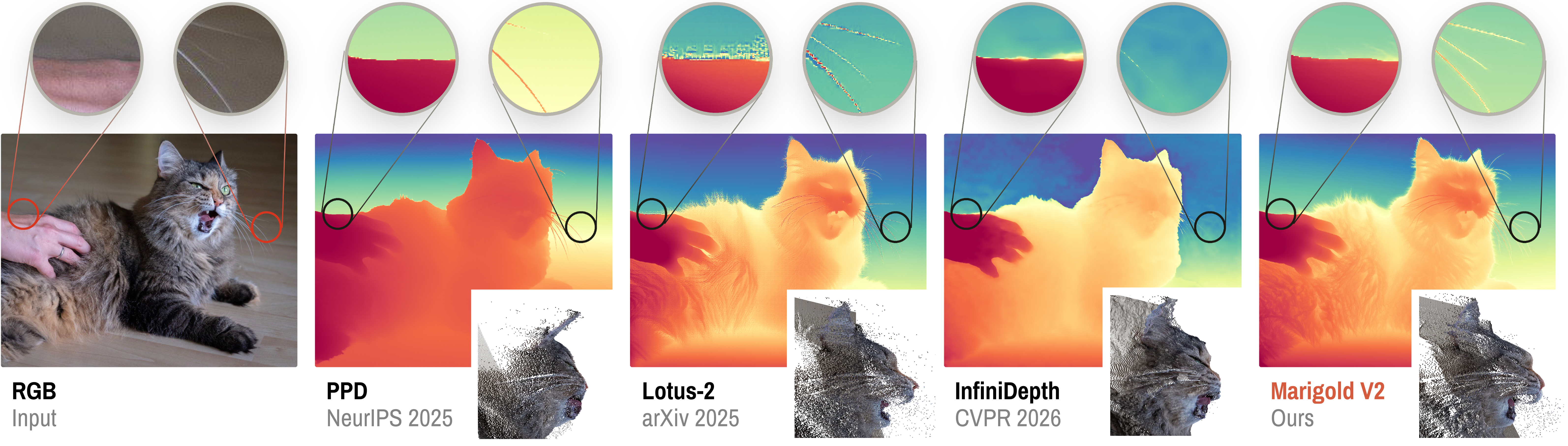
The result: 2.8 AbsRel on ETH3D (prior best 3.8), 5.4 on KITTI (prior best 6.5), and the best soft-edge-error scores against detail-specialist baselines (PPD, InfiniDepth).
The uncomfortable part first: the headline “16–26%” framing is measured against FE2E on the two datasets where the gain is largest. On NYUv2 the improvement over FE2E is 3.8 → 3.6 AbsRel (~5%), and π³ — an ICLR 2026 method trained on >9M samples — is competitive or better on several columns. The honest claim is “state of the art among methods trained on ~74K samples, by a wide margin, and competitive with 100×-data methods.” The paper’s own table supports that reading; the abstract’s framing is the optimistic slice of it.
2. The problem, and why generative priors keep getting used for it
Monocular depth estimation asks for per-pixel depth from a single RGB image. It is ill-posed by construction: an infinite family of 3D scenes projects to the same 2D image. There is no geometric constraint to exploit the way stereo or multi-view does; the only way out is prior knowledge about how scenes are typically shaped.
Deep learning reframed this as regression from appearance features. That works, but the paper identifies a structural ceiling:
discriminative models “suffer significant drops in accuracy in corner cases that are underrepresented in the training distribution.”
The root cause is data scarcity in the right modality. Ground-truth depth requires depth sensors or synthetic rendering. Both are limited:
- Sensor data carries noise and systematic failure on non-Lambertian, transparent, or reflective surfaces — exactly the surfaces that are hard.
- Synthetic data is clean in aggregate but, as the paper shows in Figure 4, is not clean at thin structures: HyperSim’s renderer uses stochastic sampling, so hair-thin geometry appears semi-transparent in RGB and ill-defined in the depth buffer.
Generative diffusion models, by contrast, are trained on billion-scale image data and — the argument goes — internalize “a geometrically consistent representation of the world” as a side effect of learning to synthesize plausible images. The bet of the whole Marigold line is that this prior is worth more than 100× more depth labels.
The bet has a known failure mode, which the paper is explicitly organized around:
“loss of fine-grained details and oversmoothed boundaries in predicted depth maps”
Every diffusion-derived depth estimator has fought this. Marigold V2’s two novel losses are both attacks on it.
3. Where this sits in the literature
3.1 Discriminative monocular depth
Three generations:
- Single-domain models trained with ground truth, self-supervision, or proxy annotations. No cross-dataset generalization.
- Affine-invariant, mixed-dataset models — the MiDaS lineage — which achieve zero-shot cross-dataset transfer by giving up absolute scale and shift.
- ViT + million-scale models: Depth Anything V1/V2, MoGe, MoGe-2, π³, spanning affine-invariant, universal metric, and video depth.
These are strong. MoGe-2 and π³ appear in Table 1 and are not embarrassed by Marigold V2. The paper’s criticism is about annotation supply and quality, not about architecture.
3.2 Generative priors
The paper sorts prior work into three families:
| Family | Characteristic | Cost |
|---|---|---|
| Multi-step diffusion preserved | Highest quality, iterative refinement | Expensive at inference |
| Single-pass distillation | Trades quality for speed | Cheap inference, detail loss |
| Architecture departures | Auxiliary inputs, extended VAE outputs | Varies |
The historical arc: early work (Marigold V1, GeoWizard, DepthFM) built on Stable Diffusion’s convolutional U-Net. The generative community then migrated to Diffusion Transformers — PixArt-α, SD3, FLUX, Qwen — and repurposing became “costlier due to the higher complexity of DiTs.”
The concrete cost numbers the paper cites are the motivation for the entire contribution:
- DICEPTION: 96 GPU-days
- Lotus-2: 8 GPUs
Note that LoRA alone does not solve this. The paper is explicit that “parameter-efficient methods like LoRA don’t always reduce this burden.” The memory wall is the frozen base weights in fp16/bf16, not the optimizer state. This is why the Q in QLoRA is load-bearing here, not incidental.
3.3 Representation alignment
REPA and iREPA showed that regularizing diffusion internals against a pretrained visual encoder improves “semantic fidelity and training convergence.” Applied to depth:
- DepthMaster: aligns intermediate U-Net features with DINOv2 features of the input image.
- Pixel-Perfect Depth: injects semantic representations via a Semantics-Prompted DiT.
Marigold V2 inverts the target:
iREPA-depth “draws its alignment target from a frozen DINOv3 encoder applied to the ground-truth depth map rather than the input image.”
Two consequences, both stated by the authors:
- It gives a “more direct supervisory signal for geometric reconstruction” — you are asking the DiT’s internals to look like the semantics of the answer, not of the question.
- It has no inference-time dependency. The DINOv3 encoder is a training-time-only object. DepthMaster-style RGB alignment likewise doesn’t need it at inference, but Semantics-Prompted approaches do; iREPA-depth stays free.
3.4 Detail and artifact handling
The paper’s survey of the detail problem, and why each prior fix is partial:
| Method | Approach | Residual problem |
|---|---|---|
| SharpDepth | Distills boundary sharpness | Predictions “remain over-smoothed” |
| InfiniDepth | Neural implicit field, arbitrary-resolution query | Resolution ≠ detail |
| Lotus-2 | Predictor–sharpener design | Requires multi-step inference |
| Pixel-Perfect Depth (PPD) | Pixel-space diffusion | Reduces flying pixels but “doesn’t recover fine detail” |
The claimed gap:
“no existing approach jointly addresses detail preservation and robust supervision under noisy or ambiguous ground-truth within a single-step VAE-based generative framework”
This is a narrow, defensible gap statement — note how many qualifiers it carries. It is not “nobody does detail”; it is “nobody does detail and noise-robustness and single-step and VAE-based, together.”
4. Method
4.0 The pipeline at a glance
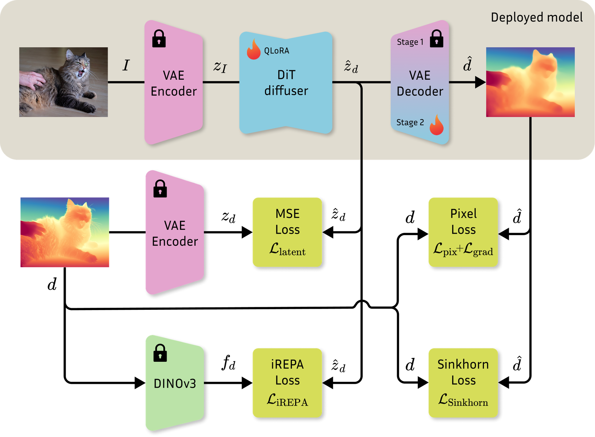
Reconstructed as a flowchart:
flowchart TB
    subgraph S1["STAGE 1 — 160K steps, ~5 days"]
        direction TB
        I1["Input image I"] --> VE1["VAE encoder ℰ_vae<br/>FROZEN"]
        GT1["Normalized GT depth d<br/>(3-channel grayscale)"] --> VE1
        VE1 --> ZI1["z_I = ℰ_vae(I)"]
        VE1 --> ZD1["z_d = ℰ_vae(d)"]
        ZI1 --> DIT1["DiT f_θ<br/>Qwen-Image-Edit-2509<br/>4-bit base + rank-128 LoRA<br/>TRAINABLE (adapters only)"]
        ZD1 --> VTGT["target velocity<br/>v = z_I − z_d"]
        DIT1 --> PRED1["f_θ(z_I, t=0.5)"]
        PRED1 --> LLAT["ℒ_latent = ‖f_θ(z_I,t) − v‖²₂"]
        VTGT --> LLAT
        PRED1 --> DEC1["VAE decoder 𝒟_vae<br/>FROZEN"]
        DEC1 --> DHAT1["d̂"]
        DHAT1 --> LPIX["ℒ_pix (L1)"]
        DHAT1 --> LGRAD["ℒ_grad (L1 on ∇x, ∇y)"]
        DIT1 -.->|internal features| LIREPA["ℒ_iREPA"]
        GT1 --> DINO["DINOv3 encoder<br/>FROZEN<br/>applied to GT DEPTH"]
        DINO --> LIREPA
    end

    S1 ==> CKPT["Stage-1 checkpoint<br/>(already SOTA-competitive)"]

    subgraph S2["STAGE 2 — 30K steps, ~1 day"]
        direction TB
        CKPT2["Stage-1 weights"] --> DIT2["DiT f_θ<br/>QLoRA adapters<br/>TRAINABLE"]
        DIT2 --> DEC2["VAE decoder 𝒟_vae<br/>UNFROZEN — TRAINABLE"]
        DEC2 --> DHAT2["d̂"]
        DHAT2 --> SINK["ℒ_SinkLoss<br/>Sinkhorn OT on 5×5 blocks"]
        DIT2 -.->|internal features| LIREPA2["ℒ_iREPA (retained, λ=0.2)"]
    end

    CKPT ==> S2
    S2 ==> FINAL["Marigold V2"]

    style S1 fill:#e8f0fe,stroke:#4a6fa5
    style S2 fill:#fdf0e8,stroke:#a56f4a
    style FINAL fill:#e8f5e9,stroke:#4a8f5a
And the inference path, which is deliberately trivial — one VAE encode, one DiT forward, one VAE decode:
flowchart LR
    I["RGB image I"] --> E["ℰ_vae"]
    E --> ZI["z_I"]
    ZI --> F["DiT f_θ<br/>single forward pass<br/>t = 0.5"]
    F --> V["predicted velocity"]
    ZI --> SUB(("−"))
    V --> SUB
    SUB --> ZD["ẑ_d = z_I − f_θ(z_I, t)"]
    ZD --> D["𝒟_vae"]
    D --> OUT["d̂ — affine-invariant log-depth"]

    style F fill:#e8f0fe,stroke:#4a6fa5
    style OUT fill:#e8f5e9,stroke:#4a8f5a
No iterative denoising. No ensembling over noise seeds (Marigold V1’s expensive trick). No DINOv3 at inference. This is the efficiency claim.
4.1 Depth normalization
Metric depth D is mapped to an affine-invariant log-depth target d:
\[ d = 2\left[\frac{\log(D+\varepsilon) - d_{2}}{d_{98} - d_{2}} - \frac{1}{2}\right] \]
| Symbol | Meaning |
|---|---|
| \(D\) | Metric ground-truth depth |
| \(\varepsilon\) | Small constant preventing \(\log(0)\) |
| \(d_{2}, d_{98}\) | 2nd and 98th percentiles of \(\log(D+\varepsilon)\) over valid pixels only |
| \(d\) | Normalized target, range \([-1, 1]\) |
Three design decisions are packed into this one line:
- Log space. Table 4 is the justification — log-depth beats both linear depth and disparity (4.72 vs 5.04 vs 5.28 AbsRel). This is not arbitrary: AbsRel is a relative error metric, so an L1 loss in log space is approximately an L1 loss on relative error, which aligns the training objective with the evaluation metric. Linear-depth L1 over-weights far pixels; disparity over-weights near ones.
- Percentile clipping, not min/max. Using \(d_2\)/\(d_{98}\) rather than the extremes makes normalization robust to a handful of sensor outliers or sky pixels that would otherwise compress the entire usable range.
- Affine invariance. Discarding absolute scale and shift is what makes cross-dataset training possible at all — HyperSim and vKITTI have incomparable depth ranges.
Then a pragmatic trick:
“The normalized depth map is encoded as a grayscale RGB image by replicating the same normalized depth value across the three color channels.”
This is the key to reusing the pretrained VAE untouched. The VAE expects 3-channel images in \([-1,1]\); a replicated depth map is exactly that. No new encoder, no architectural surgery, and — importantly — the VAE’s learned priors about natural-image structure transfer to depth maps, which are themselves piecewise-smooth-with-sharp-edges in much the way images are.
4.2 Diffusion transformer adaptation
Base model: Qwen-Image-Edit-2509.
This choice deserves a beat. It is an image-editing model, not a text-to-image model. An editing model is already trained on the conditional task “given this image, produce a related image” — structurally the same shape as “given this image, produce its depth map.” The conditioning pathway already exists and is already aligned to spatial correspondence with the input. That is a materially easier starting point than a T2I model, where the image-conditioning path has to be grafted on.
Components:
| Component | Role | Stage 1 | Stage 2 |
|---|---|---|---|
| \(\mathcal{E}_{vae}\) | VAE encoder | Frozen | Frozen |
| \(f_\theta\) | DiT backbone | 4-bit quantized base + trainable rank-128 LoRA | Trainable LoRA |
| \(\mathcal{D}_{vae}\) | VAE decoder | Frozen | Unfrozen / trainable |
Forward formulation. Both image and depth are encoded into the shared latent space:
\[ z_I = \mathcal{E}_{vae}(I), \qquad z_d = \mathcal{E}_{vae}(d) \]
The DiT is trained to regress the velocity between them:
\[ v = z_I - z_d \]
\[ \mathcal{L}_{latent} = \lVert f_\theta(z_I, t) - v \rVert_2^2 \]
at a fixed timestep \(t = 0.5\).
This is the crucial simplification, and it is worth being precise about what it means. In flow-matching / rectified-flow training you would sample \(t \sim \mathcal{U}[0,1]\) and learn the velocity field along the whole trajectory, then integrate at inference. Here the model is trained at a single point on the trajectory and the “ODE integration” collapses to one Euler step of size 1:
\[ \hat{z}_d = z_I - f_\theta(z_I, t) \]
\[ \hat{d} = \mathcal{D}_{vae}(\hat{z}_d) \]
So this is not really a diffusion model at inference. It is a deterministic feed-forward regressor that inherits diffusion-pretrained weights. The generative machinery is a weight-initialization and architecture story, not a sampling story. (This is a continuation of what Lotus and GenPercept established: for a deterministic dense-prediction target, the stochasticity of diffusion is a cost, not a benefit.)
Pixel-space auxiliary losses. Because the decode path is differentiable, supervision can be applied after decoding rather than only in latent space:
\[ \mathcal{L}_{pix} = \lVert \hat{d} - d \rVert_1 \]
\[ \mathcal{L}_{grad} = \lVert \nabla_x \hat{d} - \nabla_x d \rVert_1 + \lVert \nabla_y \hat{d} - \nabla_y d \rVert_1 \]
\(\mathcal{L}_{grad}\) is the classic multi-scale-gradient idea: penalizing gradient mismatch directly supervises edges, which an L1-on-values loss under-weights (an edge is a tiny fraction of pixels). Its weight is \(\lambda_{grad} = 5.0\) — five times the value losses — which tells you how much the authors are willing to pay for boundary fidelity.
4.3 iREPA-depth: semantic regularization from the answer, not the question
“We regularize the internal DiT representations using pretrained visual features, encouraging the model to also preserve semantically-meaningful structure.”
Mechanism: a frozen DINOv3 encoder produces target features; the DiT’s internal representations are aligned to them.
The inversion: targets come from the ground-truth depth map, not the RGB image.
The ablation is the argument. From Table 3 at 30K steps:
| Configuration | NYUv2 | KITTI | ETH3D | ScanNet | DIODE |
|---|---|---|---|---|---|
| \(\mathcal{L}_{latent} + \mathcal{L}_{pix}\) | 4.70 | 7.84 | 4.32 | 4.50 | 6.22 |
| \(+\ \mathcal{L}_{iREPA}^{rgb}\) | 4.50 | 6.89 | 3.64 | 4.38 | 5.72 |
| \(+\ \mathcal{L}_{iREPA}^{depth}\) | 4.36 | 6.72 | 3.62 | 4.22 | 5.55 |
iREPA-depth wins on all five datasets against iREPA-rgb. Not by much — ~1–3% relative — but monotonically, which is more convincing than a large win on one benchmark.
Why it should work. DINOv3 features of a depth map encode “what regions are coherent objects with coherent geometry.” Asking the DiT’s internals to match those features is asking it to have an internal object/surface decomposition of the thing it is predicting. RGB features encode object identity and texture — informative, but they also encode things depth should ignore (albedo, shadows, print on a surface), which is arguably why the RGB variant is measurably worse.
LPIPS is the natural baseline here because it is also a pretrained-feature-space loss — the comparison isolates which feature space, not whether to use one.
Stage-1 total objective:
\[ \mathcal{L}_{DiT} = \lambda_{latent}\mathcal{L}_{latent} + \lambda_{pix}\mathcal{L}_{pix} + \lambda_{grad}\mathcal{L}_{grad} + \lambda_{iREPA}\mathcal{L}_{iREPA} \]
| Coefficient | Value |
|---|---|
| \(\lambda_{latent}\) | 1.0 |
| \(\lambda_{pix}\) | 1.0 |
| \(\lambda_{grad}\) | 5.0 |
| \(\lambda_{iREPA}\) | 0.2 |
NOT STATED in the recoverable text: which DINOv3 variant (ViT-S/B/L/H), which DiT block the alignment is taken from, and what projection head maps DiT feature dimension to DINOv3 feature dimension. REPA-family work conventionally uses an early-to-middle block and a small MLP projector, but do not assume this — check the released code before reimplementing.
4.4 SinkLoss: refusing to fit the noise
This is the paper’s most interesting contribution, and the one most likely to transfer to other problems.
The problem
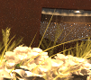
Figure 4 shows a HyperSim crop at native resolution. The caption:
“Thin structures appear semi-transparent in RGB and are not well-defined in ground-truth depth due to stochastic sampling within the rendering pipeline.”
The authors then state the trap directly:
“To achieve the best AbsRel and δ₁ scores, predictions would have to align perfectly with the ground truth and reproduce that noise.”
Sit with that. At a hair-thin structure, the “correct” per-pixel answer in the label is partly a rendering artifact. A pixel-wise loss makes the model’s incentive to reproduce the artifact. You can either have a sharp, physically plausible prediction or a low pixel-wise loss — not both. Every prior detail-focused method has been fighting the optimizer over this.
The move
Relax spatial correspondence within a small neighborhood. Tile the image into non-overlapping K×K blocks (K = 5). Within each block, allow the K² predicted values to be matched to the K² ground-truth values by an optimal permutation rather than the identity permutation.
The model is then scored on whether it produced the right multiset of depth values in this neighborhood, not whether each value landed on exactly the right pixel. Sub-block spatial jitter — which is what rendering noise looks like — becomes free. Getting the distribution wrong — an over-smoothed blob where there should be a thin bright line — remains expensive.
flowchart TB
    A["Predicted d̂ and GT d"] --> B["Tile into non-overlapping<br/>K×K blocks, K = 5"]
    B --> C["Per block: 25 predicted values,<br/>25 ground-truth values"]
    C --> D["Cost matrix<br/>C_ij = |d̂_i − d_j|<br/>(25 × 25)"]
    D --> E{"Validity mask<br/>m_i · m_j = 1 ?"}
    E -->|yes| F["C̃_ij = C_ij"]
    E -->|no| G["C̃_ij = B = 10⁶<br/>penalizes whole row AND column"]
    F --> H["Entropic OT:<br/>M = argmin ⟨M,C̃⟩ − τ·H(M)<br/>τ = 0.1, uniform marginals 1/K²"]
    G --> H
    H --> I["Sinkhorn–Knopp,<br/>5 iterations,<br/>log domain for stability"]
    I --> J["ℒ = Σ m_i m_j M_ij C_ij / Σ m_i m_j M_ij"]
    J --> K["Average over blocks<br/>with valid ground truth"]

    style H fill:#e8f0fe,stroke:#4a6fa5
    style K fill:#e8f5e9,stroke:#4a8f5a
The formulation
Cost matrix (Eq. 8). For predicted value \(i\) and ground-truth value \(j\) within a block:
\[ C_{ij} = \lvert \hat{d}_i - d_j \rvert \]
Invalid pixels are handled by a masked variant:
\[ \tilde{C}_{ij} = \begin{cases} C_{ij} & \text{if } m_i m_j = 1 \\ B & \text{otherwise}, \quad B \gg \max_{ij} C_{ij} \end{cases} \]
with \(B = 10^6\). Setting the whole row and column to a prohibitive cost means the transport solver will route mass away from invalid pixels on both sides — invalid predictions don’t get matched to valid targets and vice versa.
Entropic optimal transport (Eq. 9):
\[ M = \arg\min_{M \in \mathcal{U}} \langle M, \tilde{C} \rangle - \tau H(M) \]
| Symbol | Meaning |
|---|---|
| \(\mathcal{U}\) | Transport polytope with uniform marginals: \(M\mathbf{1} = \mathbf{1}/K^2\), \(M^\top\mathbf{1} = \mathbf{1}/K^2\) |
| \(H(M) = -\sum_{ij} M_{ij}\log M_{ij}\) | Shannon entropy of the transport plan |
| \(\tau = 0.1\) | Entropic regularization strength |
The entropy term is what makes this tractable and differentiable. Exact optimal transport over a 25×25 cost matrix is a linear program — solvable, but with no useful gradient (the solution is a vertex of the polytope; the argmin is piecewise constant). Adding \(-\tau H(M)\) makes the objective strictly convex, the solution unique and interior, and — critically — the Sinkhorn–Knopp fixed point differentiable by unrolling.
The loss (Eq. 10):
\[ \mathcal{L}_{SinkLoss} = \frac{\sum_{ij} m_i m_j M_{ij} C_{ij}}{\sum_{ij} m_i m_j M_{ij}} \]
A mass-weighted mean transport cost over valid pairs, normalized so that blocks with many invalid pixels are not systematically down-weighted. Averaged over all blocks containing valid ground truth.
Hyperparameters:
| Parameter | Value | Interpretation |
|---|---|---|
| \(K\) | 5 | Block edge → 25×25 cost matrix, ±2 px of permitted jitter |
| \(\tau\) | 0.1 | Entropic regularization |
| \(B\) | \(10^6\) | Invalid-pixel penalty |
| Sinkhorn iterations | 5 | Very few — see below |
| Computation | Log domain | Numerical stability |
On the choice of 5 iterations. This is remarkably few; Sinkhorn is usually run to convergence (tens to hundreds of iterations). Two readings, both plausible: (a) at \(\tau = 0.1\) on a 25×25 problem with uniform marginals, the plan is close enough after 5 sweeps that further iterations don’t change the gradient meaningfully; (b) it is a deliberate compute/memory budget, since the unrolled iterations must be held in the autograd graph for every block in the image. Either way, 5 unrolled iterations per block per step is the real cost, and it is why SinkLoss is a Stage-2 refinement rather than a Stage-1 objective — running it for all 160K steps would be wasteful.
On K = 5. The block size is the single most important knob and it is a genuine tradeoff: larger K tolerates more label noise but also forgives real localization error. K = 5 permits roughly ±2 pixels of positional slop. That is the scale of the rendering artifacts in Figure 4 and small enough that a mislocalized object boundary is still penalized. Non-overlapping tiling also means the block grid is arbitrary relative to image content — a boundary falling on a tile edge gets no benefit. Overlapping blocks would fix this at real compute cost; the paper takes the cheap option.
Why unfreeze the VAE decoder in Stage 2
SinkLoss operates in pixel space, after decoding. If the VAE decoder is frozen, the decoder itself becomes the bottleneck on achievable sharpness — the DiT can produce a perfect latent and the frozen decoder will still band-limit it, because it was trained to reconstruct natural images, not depth maps.
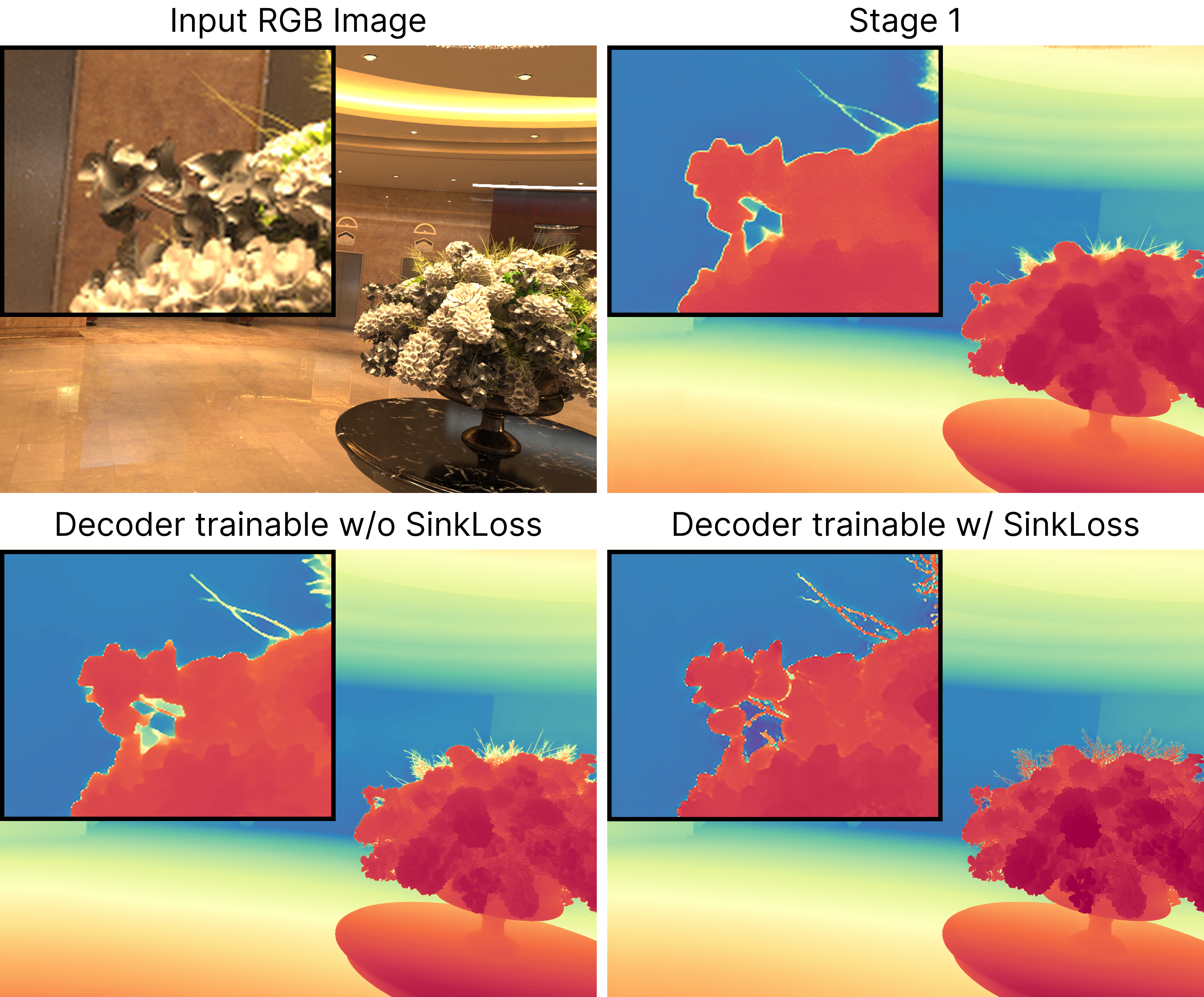
Figure 5’s caption confirms these were ablated as separate factors:
“The Stage-1 checkpoint is compared against two continued-training variants with an unfrozen VAE decoder, with and without SinkLoss. SinkLoss substantially reduces flying pixels while preserving fine detail.”
So the comparison isolates SinkLoss given an unfrozen decoder — decoder unfreezing alone is not credited with the improvement.
Stage-2 objective weights:
| Coefficient | Value |
|---|---|
| \(\lambda_{iREPA}\) | 0.2 (retained from Stage 1) |
| \(\lambda_{SinkLoss}\) | 1.0 |
[Guessing] Whether \(\mathcal{L}_{latent}\), \(\mathcal{L}_{pix}\), \(\mathcal{L}_{grad}\) are retained in Stage 2 is not stated in the recoverable text; only the two coefficients above are given. Dropping the pixel-wise terms entirely would be consistent with the motivation (they are the terms that force noise-fitting), but the paper does not say.
5. Training setup
| Aspect | Value |
|---|---|
| Base model | Qwen-Image-Edit-2509 |
| Adaptation | QLoRA — 4-bit base quantization, rank-128 adapters |
| Training data | HyperSim (filtered to <0.1% invalid pixels) + vKITTI |
| Sampling ratio | 90% HyperSim / 10% vKITTI per batch |
| Resolution | HyperSim 768×512; vKITTI 1216×352 |
| Batch size | 1 |
| Gradient clipping | Yes (value not stated) |
| Hardware | Single 32 GB GPU |
| Stage 1 | 160,000 steps, ~5 days |
| Stage 2 | 30,000 steps, ~1 day |
| Total | ~190K steps, ~6 days, ~74K training samples |
| Inference resolution | Native, except ETH3D at 1008×672 upsampled to 2048×1360 |
NOT STATED: optimizer, learning rate, LR schedule, warmup, weight decay, EMA, whether test-time ensembling is used. These are material for reproduction. Get them from the released code.
Observations worth making:
Batch size 1 with 190K steps is a memory-constrained choice, not a principled one. With rank-128 adapters and no gradient accumulation mentioned, gradient estimates are extremely noisy — which is probably why gradient clipping is called out explicitly and why the step count is so high. If you have more VRAM, accumulation is the first thing to try.
The 90/10 HyperSim/vKITTI mix is heavily indoor-synthetic. HyperSim is indoor scenes; vKITTI is synthetic driving. There is no real-world data in training at all, and no outdoor-natural data. That the model then tops KITTI (real driving) and ETH3D (real, mixed) zero-shot is the generative-prior argument working — but it also means the model has never seen a real sensor’s noise characteristics.
~74K training samples against Depth Anything V2’s 62.6M and π³’s >9M. This is the number to keep in mind when reading Table 1.
6. Results
6.1 Zero-shot affine-invariant depth (Table 1)
Metrics: AbsRel (mean absolute relative error, ↓) and δ₁ (% of pixels within a 1.25× factor of ground truth, ↑). Evaluation uses RANSAC-based robust alignment to ground-truth metric depth before computing metrics, following the Pixel-Perfect Depth protocol.
| Method | Train data | NYUv2 AbsRel↓ | NYUv2 δ₁↑ | KITTI AbsRel↓ | KITTI δ₁↑ | ETH3D AbsRel↓ | ETH3D δ₁↑ | ScanNet AbsRel↓ | ScanNet δ₁↑ | DIODE AbsRel↓ | DIODE δ₁↑ |
|---|---|---|---|---|---|---|---|---|---|---|---|
| Omnidata | 12.2M | 7.4 | 94.5 | 14.9 | 83.5 | 16.6 | 77.8 | 7.5 | 93.6 | — | — |
| DepthAnything V2 (62M) | 62.6M | 4.5 | 97.9 | 7.4 | 94.6 | 13.1 | 86.5 | 6.5 | 97.2 | 6.6 | 95.2 |
| MoGe | 9M | 3.1 | 98.3 | 7.2 | 95.1 | 10.0 | 89.6 | 3.3 | 98.3 | 29.0 | 70.0 |
| MoGe-2 | 8.9M | 3.1 | 98.4 | 6.9 | 89.9 | 5.0 | 96.2 | 3.1 | 98.3 | 9.6 | 84.5 |
| π³ † | >9M | 2.9 | 98.7 | 5.9 | 96.7 | 2.9 | 98.9 | 2.1† | 99.1† | 4.4 | 96.8 |
| DiverseDepth | 320K | 11.7 | 87.5 | 19.0 | 70.4 | 22.8 | 69.4 | 10.9 | 88.2 | — | — |
| MiDaS | 2M | 11.1 | 88.5 | 23.6 | 63.0 | 18.4 | 75.2 | 12.1 | 84.6 | — | — |
| LeReS | 354K | 9.0 | 91.6 | 14.9 | 78.4 | 17.1 | 77.7 | 9.1 | 91.7 | — | — |
| DPT | 1.4M | 9.8 | 90.3 | 10.0 | 90.1 | 7.8 | 94.6 | 8.2 | 93.4 | — | — |
| HDN | 300K | 6.9 | 94.8 | 11.5 | 86.7 | 12.1 | 83.3 | 8.0 | 93.9 | — | — |
| DepthAnything V2 (54K) | 54K | 5.4 | 97.2 | 8.6 | 92.8 | 12.3 | 88.4 | — | — | 8.8 | 93.7 |
| Marigold Depth V1 | 74K | 5.5 | 96.4 | 9.9 | 91.6 | 6.5 | 96.0 | 6.4 | 95.1 | 10.0 | 90.7 |
| GeoWizard | 280K | 5.2 | 96.6 | 9.7 | 92.1 | 6.4 | 96.1 | 6.1 | 95.3 | 12.0 | 89.8 |
| DepthFM | 63K | 5.5 | 96.3 | 8.9 | 91.3 | 5.8 | 96.2 | 6.3 | 95.4 | — | — |
| GenPercept | 90K | 5.2 | 96.6 | 9.4 | 92.3 | 6.6 | 95.7 | 5.6 | 96.5 | — | — |
| Lotus | 59K | 5.4 | 96.8 | 8.5 | 92.2 | 5.9 | 97.0 | 5.9 | 95.7 | 9.8 | 92.4 |
| Lotus-2 | 59K | 3.7 | 97.6 | 6.7 | 94.1 | 4.1 | 98.6 | 4.0 | 97.2 | 6.5 | 95.5 |
| PPD (512) | 54K | 4.3 | 97.4 | 8.0 | 93.1 | 4.5 | 97.7 | 4.5 | 97.3 | 7.0 | 95.5 |
| PPD (1024) | 125K | 4.1 | 97.7 | 7.0 | 95.5 | 4.3 | 98.0 | 4.6 | 97.2 | 6.8 | 95.9 |
| InfiniDepth | 3.1M | 4.3 | 97.6 | 8.7 | 92.3 | 6.1 | 95.4 | 4.7 | 96.9 | 6.4 | 95.8 |
| DepthMaster | 74K | 4.8 | 97.0 | 9.1 | 91.1 | 5.4 | 97.4 | 5.8 | 95.6 | 8.0 | 94.3 |
| FE2E | 71K | 3.8 | 97.6 | 6.5 | 96.0 | 3.8 | 98.7 | 4.3 | 97.1 | 5.6 | 96.4 |
| Marigold V2 (ours) | 74K | 3.6 | 98.0 | 5.4 | 97.4 | 2.8 | 99.2 | 3.7 | 97.9 | 5.2 | 97.1 |
Reading this honestly:
- Against the ~74K-sample cohort (the fair comparison — Marigold V1, DepthFM, Lotus/Lotus-2, PPD, DepthMaster, FE2E), Marigold V2 wins every single column. That is a clean result.
- The headline 16–26%. KITTI 6.5 → 5.4 vs FE2E is 17%. ETH3D 3.8 → 2.8 is 26%. NYUv2 is 3.8 → 3.6, about 5%. The abstract quotes the two best columns. Not misleading — it names KITTI and ETH3D explicitly — but do not generalize it.
- π³ is the elephant. With >9M training samples it beats Marigold V2 on NYUv2 (2.9 vs 3.6), KITTI δ₁ is close (96.7 vs 97.4 — Marigold wins), ETH3D is a near-tie (2.9 vs 2.8 — Marigold wins), ScanNet favors π³ (2.1†), DIODE favors π³ (4.4 vs 5.2). The dagger on π³’s ScanNet entry suggests a footnoted caveat (likely training-data overlap) that I could not recover. Marigold V2 is not uniformly SOTA across all methods; it is SOTA at its data scale and competitive well above it.
- MoGe’s DIODE collapse (29.0 AbsRel, 70.0 δ₁) is a nice illustration of the paper’s own framing about discriminative models and out-of-distribution corner cases.
- Improvement is largest where scenes are hardest. ETH3D and KITTI — high dynamic range, outdoor, thin structures — improve most. NYUv2 and ScanNet — indoor, textured, already near-saturated — improve least. Consistent with the claim that the contributions target detail and boundary quality specifically.
6.2 Edge-aware evaluation (Table 2)
SEE_k (Soft Edge Error): at depth discontinuities, the minimum absolute error between predicted disparity and any ground-truth disparity within a k×k patch. Lower is better.
Note that SEE and SinkLoss share a philosophy — both permit local spatial slack. That is a real methodological caveat: the training objective is structurally aligned with this evaluation metric in a way that competitors’ objectives are not. It does not invalidate the result (SEE predates this paper and is a reasonable measure of boundary quality) but it is not an independent test either.
Evaluated on the HyperSim test set:
| Method | SEE3↓ | SEE5↓ | SEE7↓ |
|---|---|---|---|
| PPD | 0.404 | 0.385 | 0.371 |
| InfiniDepth | 0.470 | 0.451 | 0.436 |
| Marigold V2 | 0.352 | 0.333 | 0.320 |
~13% better than PPD at k=3, and the margin holds across k. Only two baselines, both detail-specialists — a deliberately hard, narrow comparison.
6.3 Ablations (Table 3)
Full Stage-1 ablation:
| Configuration | NYUv2 AbsRel↓ | NYUv2 δ₁↑ | KITTI AbsRel↓ | KITTI δ₁↑ | ETH3D AbsRel↓ | ETH3D δ₁↑ | ScanNet AbsRel↓ | ScanNet δ₁↑ | DIODE AbsRel↓ | DIODE δ₁↑ |
|---|---|---|---|---|---|---|---|---|---|---|
| \(\mathcal{L}_{latent}\) (30K) | 4.53 | 97.60 | 7.26 | 94.94 | 4.25 | 98.25 | 4.59 | 97.41 | 6.82 | 95.81 |
| \(+\ \mathcal{L}_{pix}\) (30K) | 4.70 | 97.90 | 7.84 | 95.62 | 4.32 | 98.69 | 4.50 | 97.91 | 6.22 | 96.01 |
| \(+\ \mathcal{L}_{iREPA}^{rgb}\) (30K) | 4.50 | 97.81 | 6.89 | 96.22 | 3.64 | 98.86 | 4.38 | 97.65 | 5.72 | 96.54 |
| \(+\ \mathcal{L}_{iREPA}^{depth}\) (30K) | 4.36 | 98.01 | 6.72 | 96.38 | 3.62 | 98.90 | 4.22 | 97.91 | 5.55 | 96.82 |
| Stage 1, 160K (baseline) | 3.62 | 98.01 | 5.27 | 97.39 | 2.84 | 99.08 | 3.84 | 97.88 | 5.16 | 97.07 |
| Stage 1, 160K + iREPA-depth | 3.68 | 98.03 | 5.30 | 97.43 | 2.68 | 99.18 | 3.81 | 97.82 | 5.02 | 97.02 |
Three things to notice, one of them awkward:
Adding \(\mathcal{L}_{pix}\) makes AbsRel worse on NYUv2 (4.53 → 4.70), KITTI (7.26 → 7.84), and ETH3D (4.25 → 4.32), while improving δ₁ everywhere. A pixel-space L1 that hurts a pixel-space relative-error metric is counterintuitive; the most likely explanation is that L1 through a frozen decoder pulls toward decoder-reconstructible (i.e. smoother) outputs. It is included anyway, presumably because it is a prerequisite for \(\mathcal{L}_{grad}\) and the Stage-2 pixel-space machinery.
Training length dominates every loss choice. 30K → 160K steps improves NYUv2 from 4.36 → 3.62 — a bigger delta than every loss ablation combined. This is the honest summary of Table 3: the losses give a few percent; the compute gives ~17%.
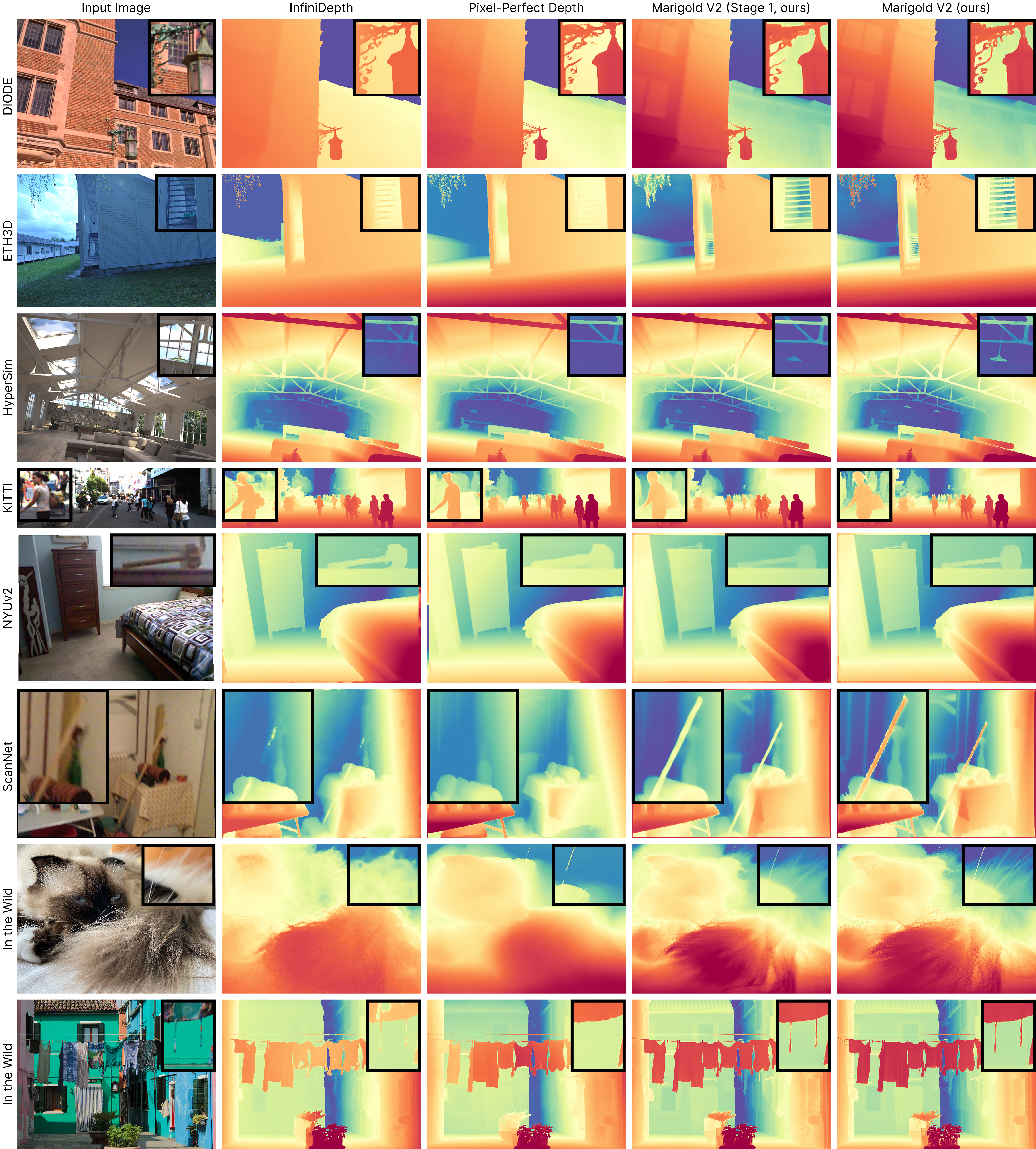
At 160K steps, iREPA-depth’s benefit is ambiguous. It worsens NYUv2 (3.62 → 3.68) and KITTI (5.27 → 5.30), and improves ETH3D (2.84 → 2.68), ScanNet (3.84 → 3.81), DIODE (5.16 → 5.02). The clean 5/5 sweep at 30K becomes 3/5 at convergence. The charitable reading — supported by Figure 3 — is that iREPA-depth buys qualitative detail and artifact removal that AbsRel does not measure. The skeptical reading is that its quantitative contribution largely washes out with sufficient training. Both readings are available from the paper’s own table, and the paper does not, in the recoverable text, address the regression.
6.4 Depth parameterization (Table 4)
Average across test sets, common training/eval configuration:
| Representation | AbsRel↓ | δ₁↑ |
|---|---|---|
| Linear depth | 5.04 | 97.10 |
| Disparity | 5.28 | 97.15 |
| Log depth | 4.72 | 97.71 |
Log depth wins on both metrics. A ~6% AbsRel gain for a change of variables — cheap, and the kind of detail that is easy to get wrong in a reimplementation.
7. Other dense regression tasks (Section 5)
Coverage gap. The body of Section 5 was not recoverable from the HTML rendering available to me. What follows is bounded by the subsection titles and the abstract’s general claim. No datasets, baselines, or numbers from Section 5 are reported here, because I could not verify any. Treat this section as a pointer to read in the paper, not as a summary of it.
The paper reports that the protocol generalizes beyond depth to four additional dense-prediction tasks, and claims “state-of-the-art results when applied to other dense regression tasks.”
| §5.x | Task | What it implies about the recipe |
|---|---|---|
| 5.1 | Depth completion | Sparse depth must enter as an additional conditioning signal — a change to the input pathway, not just the target. How this is encoded is not recoverable. |
| 5.2 | See-through depth | Predicting geometry behind/through transparent surfaces. Directly targets the non-Lambertian failure mode called out in §2.1, and is the task where the generative prior should matter most. |
| 5.3 | Surface normal estimation | A 3-channel target maps naturally onto the RGB-shaped VAE input — arguably a better fit than depth’s replicated-grayscale hack. Note that SinkLoss as formulated (\(C_{ij} = \lvert\hat{d}_i - d_j\rvert\)) is scalar; a normal-map version needs a different cost (angular distance), and whether that was done is not stated. |
| 5.4 | Albedo estimation | Intrinsic image decomposition — not geometry at all. If this works, the claim is about the protocol, not about depth. |
The structural argument is sound: nothing in QLoRA adaptation, iREPA-style alignment, or block-wise OT matching is depth-specific. The evidence for it is in a section I could not read.
8. Practical notes
8.1 Using the model
The demo is at hf.co/spaces/huawei-bayerlab/marigold-v2-web.
NOT STATED in the recoverable text: whether code and weights are released, under what license, and at what repository. Check the project page before planning any work that depends on them.
Sketch of what inference looks like, given the formulation in §4.2. Illustrative, not tested — the released API will differ:
# ILLUSTRATIVE — not verified against a released implementation.
import torch

@torch.no_grad()
def predict_depth(image, vae, dit, t=0.5):
    """Single-step affine-invariant log-depth prediction.

    image: float tensor in [-1, 1], shape (B, 3, H, W)
    returns: normalized log-depth in ~[-1, 1], shape (B, 1, H, W)
    """
    z_I = vae.encode(image).latent_dist.mode()

    # One forward pass at a fixed timestep. No iterative denoising.
    v_hat = dit(z_I, timestep=t)

    # Single Euler step of size 1 along the learned velocity field.
    z_d = z_I - v_hat

    d_hat = vae.decode(z_d).sample     # (B, 3, H, W), channels are replicas
    return d_hat.mean(dim=1, keepdim=True)
Recovering metric depth requires inverting the normalization of §4.1, which needs scale and shift you do not have from a single image. That is what the RANSAC alignment in the evaluation protocol supplies:
# ILLUSTRATIVE.
import numpy as np

def to_metric(d_norm, d2, d98, eps=1e-8):
    """Invert the affine-invariant log-depth normalization.

    d2, d98 are the log-depth percentiles — NOT recoverable from the
    prediction alone. In evaluation they come from RANSAC alignment
    against ground truth; in deployment they must come from another
    source (a sparse sensor, known scene scale, or a metric model).
    """
    log_d = (d_norm / 2.0 + 0.5) * (d98 - d2) + d2
    return np.exp(log_d) - eps
This is the deployment caveat that matters. Marigold V2 is affine-invariant. It gives you relative geometry, excellently. It does not give you metres. For robotics or measurement you need a metric anchor — a few LiDAR returns, a known object size, or a separate metric model — and then the two-parameter fit.
8.2 SinkLoss, as a component you might reuse
The block-wise OT loss is the most portable idea in the paper. It applies wherever your labels are spatially noisy at fine scale but distributionally correct: segmentation boundaries, optical flow near occlusions, any sensor-derived dense target.
# ILLUSTRATIVE reference implementation of the formulation in §3.4.
# Hyperparameters follow the paper: K=5, tau=0.1, B=1e6, 5 iterations.
import torch
import torch.nn.functional as F

def sinkhorn_log(log_K, n_iters=5):
    """Sinkhorn-Knopp in the log domain, uniform marginals 1/n."""
    n = log_K.shape[-1]
    log_mu = torch.full(log_K.shape[:-1], -torch.log(torch.tensor(float(n))),
                        device=log_K.device)
    f = torch.zeros_like(log_mu)
    g = torch.zeros_like(log_mu)
    for _ in range(n_iters):
        f = log_mu - torch.logsumexp(log_K + g.unsqueeze(-2), dim=-1)
        g = log_mu - torch.logsumexp(log_K + f.unsqueeze(-1), dim=-2)
    return log_K + f.unsqueeze(-1) + g.unsqueeze(-2)   # log transport plan


def sink_loss(pred, target, mask, K=5, tau=0.1, big=1e6, n_iters=5):
    """pred/target/mask: (B, 1, H, W). mask is 1 for valid pixels."""
    # Tile into non-overlapping K x K blocks -> (B*nblocks, K*K)
    def blocks(x):
        return F.unfold(x, kernel_size=K, stride=K).transpose(1, 2).reshape(-1, K * K)

    p, t, m = blocks(pred), blocks(target), blocks(mask)

    C = (p.unsqueeze(-1) - t.unsqueeze(-2)).abs()        # (N, K^2, K^2)
    valid = (m.unsqueeze(-1) * m.unsqueeze(-2)) > 0.5
    C_tilde = torch.where(valid, C, torch.full_like(C, big))

    log_M = sinkhorn_log(-C_tilde / tau, n_iters=n_iters)
    M = log_M.exp()

    w = M * valid                                        # mask-weighted plan
    num = (w * C).sum(dim=(-2, -1))
    den = w.sum(dim=(-2, -1)).clamp_min(1e-12)

    has_gt = valid.any(dim=(-2, -1))
    return (num / den)[has_gt].mean()
Two things to watch if you adopt this: memory is \(O(N_{blocks} \cdot K^4 \cdot n_{iters})\) once unrolled for autograd — the reason K is small and iterations are few — and the non-overlapping grid means boundaries landing on a tile edge get no tolerance benefit.
8.3 Reproduction checklist
If you are reimplementing, these are the details most likely to cost you a week:
9. Critical assessment
What is genuinely strong
The cost story is the contribution. 96 GPU-days → 6 single-GPU-days, with better results, is the kind of result that changes who can do this work. It is also the claim easiest to verify and hardest to argue with.
SinkLoss is a real idea, not a trick. “Your labels are noisy at fine scale, so stop demanding pixel-exact agreement and demand distributional agreement in a small neighborhood instead” is a clean, transferable insight with a principled implementation. It correctly identifies that the metric and the objective were fighting each other, and resolves it in the objective rather than by relabeling.
The iREPA-depth inversion is a good, cheap idea with a clean ablation at 30K steps and no inference cost.
Choosing an image-editing base model rather than a T2I one is an underrated decision that probably contributes more than it gets credit for.
What to hold at arm’s length
The 16–26% framing is the best two of five columns. The median improvement over FE2E is closer to 10%.
iREPA-depth’s contribution at convergence is not established. It regresses two of five datasets at 160K steps. The paper’s quantitative case for it rests on the 30K-step ablation; its case at full training is qualitative (Figure 3).
SEE and SinkLoss are philosophically aligned. Both permit local spatial slack. Winning SEE with an objective built on the same relaxation is weaker evidence than winning a metric that does not share the assumption.
No real-world training data at all. HyperSim + vKITTI are both synthetic. Zero-shot transfer to real benchmarks works, which is the point — but the model has never seen a real depth sensor’s noise, and the benchmark suite may not surface what that costs.
π³ exists. With ~120× the data it is better on several columns. “SOTA at this data scale” is the accurate claim.
Table 2 has two baselines. Defensible (they are the right two) but thin.
Reproducibility is gated on the code release. Optimizer, LR schedule, DINOv3 variant, and iREPA layer are all unstated in the paper, and all of them matter.
Open questions
- Does SinkLoss transfer to real sensor noise (LiDAR dropout, ToF multipath) rather than only to rendering noise? The motivation generalizes; the evidence does not yet.
- What does the K-vs-tolerance curve look like? K=5 is asserted, never ablated in the recoverable text.
- Would overlapping blocks, or a random block-grid offset per step, remove the tile-boundary artifact cheaply?
- Does the single-step formulation cap achievable detail relative to a few-step variant? The paper does not report a multi-step ablation of its own model.
- How much of the gain comes from Qwen-Image-Edit specifically versus the losses? There is no base-model ablation.
10. One-paragraph summary
Marigold V2 fine-tunes Qwen-Image-Edit-2509 into a single-step affine-invariant monocular depth estimator using QLoRA (4-bit base, rank-128 adapters), a fixed-timestep velocity-regression objective, and two novel losses: iREPA-depth, which aligns DiT internals to frozen DINOv3 features computed on the ground-truth depth map, and SinkLoss, an entropic-OT matching loss over 5×5 blocks that scores predictions on the local multiset of depth values rather than per-pixel agreement, deliberately decoupling training from rendering noise at thin structures. Trained in two stages — 160K steps with the decoder frozen, then 30K with it unfrozen and SinkLoss active — for about six days on a single 32 GB GPU and ~74K synthetic samples, it beats every comparably-sized-data method on all five standard benchmarks and leads detail-specialist baselines on soft-edge error. The efficiency result is the durable contribution; SinkLoss is the idea most worth stealing; the headline percentage is the optimistic slice of the table.