Introduction and Historical Context
LeNet is the name given to a series of convolutional neural network (CNN) architectures developed primarily by Yann LeCun, along with collaborators Léon Bottou, Yoshua Bengio, and Patrick Haffner, during their time at AT&T Bell Laboratories in the late 1980s and 1990s. The work culminated in the landmark 1998 paper:
“Gradient-Based Learning Applied to Document Recognition” Yann LeCun, Léon Bottou, Yoshua Bengio, Patrick Haffner Proceedings of the IEEE, 86(11):2278–2324, November 1998.
This paper is one of the most cited papers in the history of machine learning, and it laid the groundwork for the deep learning revolution that would come a decade later with AlexNet (2012).
To appreciate why LeNet was so significant, we need to understand the intellectual and technical landscape of the late 1980s. At the time:
- Neural networks had been largely abandoned by the research community following the XOR crisis and the AI winter of the 1970s. The backpropagation algorithm had been rediscovered and popularized in the mid-1980s, but large networks were considered computationally infeasible.
- Handcrafted feature engineering dominated machine learning. Researchers would spend enormous effort designing domain-specific features (edge detectors, texture descriptors, shape descriptors) that would then be fed into simpler classifiers like SVMs or decision trees.
- Document recognition systems in production (for postal sorting, bank check reading, etc.) relied on brittle pipelines of hand-tuned components: preprocessing, segmentation, feature extraction, and classification were all separate, manually-engineered stages.
LeCun’s insight was bold and counterintuitive: instead of engineering features by hand, you could learn them directly from raw pixel data if you could design the right architecture and train it end-to-end using gradient descent. The convolutional structure he proposed was inspired by work on the visual cortex by Hubel and Wiesel (1962), who had shown that neurons in the cat visual cortex respond to small, local regions of the visual field — a property now captured by the concept of a receptive field.
LeNet showed, convincingly and at scale, that a neural network with the right inductive biases (locality, weight sharing, spatial hierarchy) could learn robust, generalizable feature representations directly from pixels. It was deployed commercially by AT&T and later NCR to read millions of handwritten checks per day, representing one of the first large-scale industrial deployments of a learned deep network.
What Problem Was LeNet Solving?
The primary application driving LeNet’s development was optical character recognition (OCR), specifically the recognition of handwritten and printed digits. The concrete use case was reading the dollar amounts and account numbers on bank checks automatically.
This is a classification problem: given a 32×32 grayscale image of a single digit (0–9), output the correct digit class.
While this may sound simple today, in the early 1990s it was genuinely hard. Handwritten digits exhibit enormous variability:
- Stroke width varies (thin, thick)
- Tilt and rotation vary (upright, slanted left or right)
- Scale varies (small, large)
- Writing style varies (cursive-like 7s, looped 9s, etc.)
- Noise from scanning and thresholding
A system achieving sub-1% error rate on a large, diverse dataset of handwritten digits was considered state-of-the-art — and that is precisely what LeNet-5 achieved on the MNIST dataset (Mixed National Institute of Standards and Technology).
Beyond digit recognition, LeCun framed this work more ambitiously as a proof of concept for end-to-end learning from raw data — a paradigm that would ultimately replace hand-engineering across virtually every domain of perception.
The LeNet Family: From LeNet-1 to LeNet-5
The name “LeNet” loosely refers to a family of related architectures developed over roughly a decade:
timeline
    title LeNet Family History
    1989 : LeNet-1
         : 16×16 input
         : ~2,600 parameters
         : Zip code recognition paper
    1993 : LeNet-4
         : Larger feature maps
         : Improved accuracy
    1998 : LeNet-5
         : 32×32 input
         : ~61,750 parameters
         : Landmark IEEE paper
         : Deployed for bank check reading
LeNet-1 (1989)
LeCun’s first published CNN, described in “Backpropagation Applied to Handwritten Zip Code Recognition” (Neural Computation, 1989). It had:
- Input: 16×16 images
- Two convolutional layers with 4 and 12 feature maps
- Two subsampling layers
- A fully connected output layer
- ~2,600 trainable parameters
It demonstrated that convolutional networks with weight sharing could learn from raw pixel data more efficiently than fully connected networks.
LeNet-4 (1993)
An intermediate architecture not described in detail in the 1998 paper but referenced. It introduced larger feature maps and demonstrated improved accuracy.
LeNet-5 (1998)
The definitive version and the architecture most people refer to when they say “LeNet.” Described in the 1998 IEEE paper, it operates on 32×32 grayscale images and has approximately 60,000 trainable parameters. This is the architecture examined in detail throughout this guide.
Architecture Deep Dive: LeNet-5
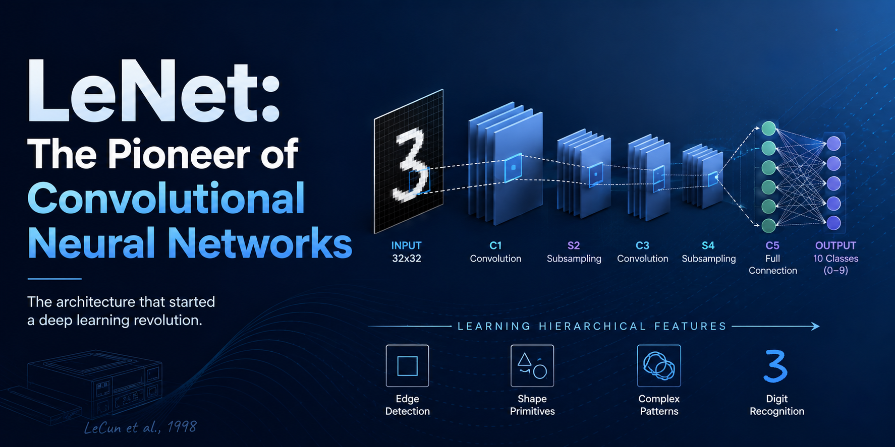
LeNet-5 is designed to take a 32×32 grayscale image as input and produce a probability distribution over 10 digit classes as output.
Here is a high-level view of the full architecture:
flowchart TD
    INPUT["🖼️ INPUT 32×32×1"]:::input
    C1["C1 — Convolutional 6 filters · 5×5 · stride 1 📐 28×28×6"]:::conv
    S2["S2 — Avg Pool 2×2 · stride 2 📐 14×14×6"]:::pool
    C3["C3 — Convolutional 16 filters · 5×5 · stride 1 📐 10×10×16"]:::conv
    S4["S4 — Avg Pool 2×2 · stride 2 📐 5×5×16"]:::pool
    C5["C5 — Convolutional 120 filters · 5×5 · stride 1 📐 1×1×120 (≡ Fully Connected)"]:::conv
    F6["F6 — Fully Connected 120 → 84 units"]:::fc
    OUT["OUTPUT — Fully Connected 84 → 10 units (Softmax)"]:::output

    INPUT --> C1 --> S2 --> C3 --> S4 --> C5 --> F6 --> OUT

    classDef input  fill:#dbeafe,stroke:#2563eb,color:#1e3a8a,font-weight:bold
    classDef conv   fill:#dcfce7,stroke:#16a34a,color:#14532d
    classDef pool   fill:#fef9c3,stroke:#ca8a04,color:#713f12
    classDef fc     fill:#f3e8ff,stroke:#9333ea,color:#3b0764
    classDef output fill:#fee2e2,stroke:#dc2626,color:#7f1d1d,font-weight:bold
Each layer is described in detail below.
Layer C1: First Convolutional Layer
| Property | Value |
|---|---|
| Type | Convolutional |
| Input | 32×32×1 |
| Kernel size | 5×5 |
| Number of filters | 6 |
| Stride | 1 |
| Padding | None (valid) |
| Output size | 28×28×6 |
| Trainable parameters | (5×5×1 + 1) × 6 = 156 |
C1 applies 6 independent 5×5 convolution kernels to the input image. Each kernel slides across the 32×32 image with a stride of 1 pixel. Because there is no padding and the kernel is 5×5, the output spatial dimensions follow:
\[ \text{output\_size} = \frac{\text{input\_size} - \text{kernel\_size}}{\text{stride}} + 1 = \frac{32 - 5}{1} + 1 = 28 \]
The result is 6 feature maps of size 28×28, visualised below:
flowchart LR
    subgraph IN["Input Image"]
        direction TB
        I["32×32×1 (grayscale)"]
    end
    subgraph K["Learned Kernel"]
        direction TB
        KK["5×5 weights + 1 bias = 26 params"]
    end
    subgraph OP["Convolution (stride 1, no pad)"]
        direction TB
        CALC["(32−5)/1+1 = 28"]
    end
    subgraph OUT["Output Feature Map"]
        direction TB
        O["28×28 (one of 6 maps)"]
    end

    IN  -->|"slide"| OP
    K   -->|"dot product"| OP
    OP  --> OUT

    style IN  fill:#dbeafe,stroke:#2563eb,color:#1e3a8a
    style K   fill:#dcfce7,stroke:#16a34a,color:#14532d
    style OP  fill:#fef9c3,stroke:#ca8a04,color:#713f12
    style OUT fill:#f3e8ff,stroke:#9333ea,color:#3b0764
Filters at this stage tend to learn low-level features: oriented edges, blobs, corners, and gradients.
All 26 parameters (5×5 weights + 1 bias) of each filter are shared across all 28×28 = 784 positions where that filter is applied. This reduces the number of parameters compared to a fully connected layer and encodes the prior belief that useful features should be detectable anywhere in the image (translation equivariance).
Layer S2: First Subsampling (Pooling) Layer
| Property | Value |
|---|---|
| Type | Average pooling (learnable in original) |
| Input | 28×28×6 |
| Pool size | 2×2 |
| Stride | 2 |
| Output size | 14×14×6 |
| Trainable parameters | 2 × 6 = 12 (original), 0 (modern) |
S2 downsamples each of the 6 feature maps by a factor of 2 in both spatial dimensions. The original LeNet-5 used a learnable average pooling: each 2×2 block is summed, multiplied by a trainable scalar, added to a trainable bias, then passed through a sigmoid.
Subsampling serves several purposes:
- Reduces spatial resolution, decreasing computation in subsequent layers.
- Increases the effective receptive field of deeper neurons.
- Provides translation invariance: small input shifts produce the same pooled output.
Layer C3: Second Convolutional Layer
| Property | Value |
|---|---|
| Type | Convolutional |
| Input | 14×14×6 |
| Kernel size | 5×5 |
| Number of filters | 16 |
| Stride | 1 |
| Output size | 10×10×16 |
| Trainable parameters (full) | (5×5×6 + 1) × 16 = 2,416 |
| Trainable parameters (sparse) | 1,516 (original paper) |
C3 applies 16 filters to the 14×14×6 feature maps from S2. Each filter produces a 10×10 output (14 − 5 + 1 = 10).
One of LeNet-5’s notable quirks is that C3’s filters are not connected to all 6 input feature maps in the original design. LeCun used a specific sparse connectivity pattern where each of the 16 filters connects to only a subset (3, 4, or 6) of the 6 input maps.
The motivation was (1) parameter reduction and (2) symmetry breaking to encourage diverse features. Most modern reproductions use full connectivity instead.
Layer S4: Second Subsampling Layer
| Property | Value |
|---|---|
| Type | Average pooling |
| Input | 10×10×16 |
| Pool size | 2×2 |
| Stride | 2 |
| Output size | 5×5×16 |
| Trainable parameters | 2 × 16 = 32 (original), 0 (modern) |
Identical in structure to S2, S4 downsamples to 5×5×16. After this layer, the spatial dimensions are small enough that the next convolution will reduce them to 1×1.
Layer C5: Third Convolutional Layer
| Property | Value |
|---|---|
| Type | Convolutional (≡ fully connected) |
| Input | 5×5×16 |
| Kernel size | 5×5 |
| Number of filters | 120 |
| Output size | 1×1×120 |
| Trainable parameters | (5×5×16 + 1) × 120 = 48,120 |
C5 is technically a convolutional layer, but because the input is exactly 5×5 and the kernel is 5×5, the output collapses to 1×1. It is mathematically identical to a fully connected layer operating on the flattened 400-dimensional vector.
LeCun used a convolutional layer here rather than a dense layer so that if the input image were larger than 32×32, C5 would produce a spatial feature map instead of a single vector — a concept now called a Fully Convolutional Network (FCN). This makes the architecture naturally adaptable to variable-size inputs.
Layer F6: Fully Connected Layer
| Property | Value |
|---|---|
| Type | Fully connected |
| Input | 120 units |
| Output | 84 units |
| Activation | Scaled tanh (original), ReLU (modern) |
| Trainable parameters | (120 + 1) × 84 = 10,164 |
F6 maps the 120-dimensional representation from C5 to an 84-dimensional vector. LeCun chose 84 because it corresponds to the number of bits in a 7×12 bitmap font for ASCII characters — allowing the network’s outputs to be interpreted as character codes.
The original activation was a scaled tanh:
\[ f(x) = A \cdot \tanh(S \cdot x), \quad A = 1.7159,\; S = \tfrac{2}{3} \]
These constants were chosen to keep output variance close to 1 and delay saturation.
Output Layer
| Property | Value |
|---|---|
| Type | Euclidean RBF (original) / Softmax (modern) |
| Input | 84 units |
| Output | 10 units |
| Trainable parameters | 840 (modern) or fixed codes (original) |
The original LeNet-5 output used Euclidean RBF units. Each output unit \(y_i\) for class \(i\) computed:
\[ y_i = \sum_j (x_j - w_{ij})^2 \]
where \(w_{ij}\) is a fixed, hand-coded ASCII bitmap pattern for digit \(i\). The class with the smallest \(y_i\) was the prediction. Modern implementations replace this with standard softmax + cross-entropy loss.
Core Concepts Explained
Convolution
Convolution is the mathematical operation at the heart of CNNs. In the discrete 2D case:
\[ (I \ast K)[i, j] = \sum_{u=0}^{m-1} \sum_{v=0}^{n-1} I[i+u,\, j+v] \cdot K[u, v] \]
In deep learning, what we call “convolution” is technically cross-correlation — the kernel is not flipped before the dot product. Since the kernel is learned, this distinction is irrelevant in practice.
Intuition: A convolutional kernel is a small “template.” Sliding it across the image and computing the dot product at each position yields a high value wherever the image locally matches the template pattern.
Subsampling / Pooling
Pooling reduces the spatial resolution of feature maps. The two most common types are:
Average pooling:
\[ y[i,j] = \frac{1}{|W|} \sum_{(u,v) \in W} x[2i+u,\; 2j+v] \]
Max pooling:
\[ y[i,j] = \max_{(u,v) \in W} x[2i+u,\; 2j+v] \]
Max pooling is preferred in modern networks because it is more tolerant of exact feature position, provides stronger non-linearity, and works better with ReLU activations. LeNet-5 originally used average pooling for probabilistic principled reasons.
Activation Functions
Scaled Hyperbolic Tangent (original LeNet):
\[ f(x) = 1.7159 \cdot \tanh\!\left(\tfrac{2}{3} x\right) \]
- Output range: \((-1.7159,\; +1.7159)\)
- Symmetric, smooth, differentiable everywhere
- Saturates for large \(|x|\) → can cause vanishing gradients
ReLU (modern replacement):
\[ f(x) = \max(0,\; x) \]
- Non-saturating for positive inputs
- Sparse activations
- Computationally cheap
- Alleviates vanishing gradients
ReLU was only established as superior after Nair & Hinton (2010) and AlexNet (2012). If implementing LeNet-5 today, always use ReLU for faster convergence.
The Mathematics of LeNet
Forward Pass
Let \(\mathbf{x}^{(0)} \in \mathbb{R}^{32 \times 32}\) be the input image. The forward pass computes:
C1:
\[ a_{k}^{C1}[i,j] = b_k^{C1} + \sum_{u=0}^{4} \sum_{v=0}^{4} W_k^{C1}[u,v] \cdot x^{(0)}[i+u, j+v], \quad k=1,\ldots,6 \]
\[ x_{k}^{C1}[i,j] = f\!\left(a_k^{C1}[i,j]\right) \]
S2:
\[ x_{k}^{S2}[i,j] = f\!\left(w_k^{S2} \cdot \sum_{u=0}^{1} \sum_{v=0}^{1} x_k^{C1}[2i+u, 2j+v] + b_k^{S2}\right) \]
C3 (full connectivity):
\[ a_{k}^{C3}[i,j] = b_k^{C3} + \sum_{m=1}^{6} \sum_{u=0}^{4} \sum_{v=0}^{4} W_{k,m}^{C3}[u,v] \cdot x_m^{S2}[i+u, j+v], \quad k=1,\ldots,16 \]
S4, C5, and F6 follow the same pattern. The final softmax output:
\[ \hat{y}_i = \frac{e^{z_i}}{\sum_{j=0}^{9} e^{z_j}} \]
Loss Function
With softmax output, the cross-entropy loss is:
\[ \mathcal{L} = -\sum_{i=0}^{9} y_i \log \hat{y}_i \]
For a single correct class \(c\), this simplifies to:
\[ \mathcal{L} = -\log \hat{y}_c = -z_c + \log \sum_j e^{z_j} \]
Parameter Count Summary
| Layer | Parameters |
|---|---|
| C1 | 156 |
| S2 | 12 |
| C3 | 2,416 |
| S4 | 32 |
| C5 | 48,120 |
| F6 | 10,164 |
| Output | 850 |
| Total | ~61,750 |
Training LeNet: Backpropagation Through Convolutions
Training a CNN requires computing gradients of the loss with respect to all trainable parameters. Convolutional layers require special treatment compared to fully connected layers.
Gradient w.r.t. Bias
\[ \frac{\partial \mathcal{L}}{\partial b_k} = \sum_{i,j} \delta_k[i,j] \]
where \(\delta_k[i,j] = \partial \mathcal{L} / \partial a_k[i,j]\) is the upstream error signal.
Gradient w.r.t. Kernel Weights
\[ \frac{\partial \mathcal{L}}{\partial W_k[u,v]} = \sum_{i,j} \delta_k[i,j] \cdot x[i+u, j+v] \]
This is the cross-correlation of the input with the upstream gradient.
Gradient w.r.t. Input
\[ \frac{\partial \mathcal{L}}{\partial x[i,j]} = \sum_k \sum_{u,v} \delta_k[i-u, j-v] \cdot W_k[u,v] \]
This is a full convolution (the kernel is flipped), not cross-correlation.
Gradient Through Pooling
Average pooling — gradient is distributed equally:
\[ \frac{\partial \mathcal{L}}{\partial x[2i+u,\, 2j+v]} = \frac{1}{4} \cdot \delta[i,j] \]
Max pooling — gradient flows only to the winning position:
\[ \frac{\partial \mathcal{L}}{\partial x[2i+u,\, 2j+v]} = \delta[i,j] \cdot \mathbf{1}\!\left[(2i+u, 2j+v) = \operatorname{argmax}\right] \]
Optimization
The original LeNet-5 used SGD with a scheduled learning rate and a diagonal Hessian approximation for adaptive rates — a precursor to modern optimizers like Adam. Modern training uses:
- SGD with momentum (typically \(\mu = 0.9\))
- Adam (adaptive per-parameter learning rates)
- Weight decay / L2 regularization
- Learning rate schedules (step decay, cosine annealing)
The MNIST Dataset and LeNet’s Performance
The MNIST dataset consists of:
- 60,000 training images of handwritten digits (0–9)
- 10,000 test images
- Each image is 28×28 pixels, grayscale, centered and normalized
For LeNet-5’s 32×32 input, MNIST images are zero-padded. The original paper normalized pixel values to \([-0.1,\; 1.175]\) (background → −0.1, foreground → 1.175).
Historical Performance on MNIST
| Method | Test Error Rate |
|---|---|
| Nearest Neighbor (raw pixels) | 5.00% |
| Linear Classifier | 7.60% |
| MLP (1 hidden layer, 300 units) | 4.50% |
| MLP (2 hidden layers) | 3.05% |
| LeNet-1 | 1.70% |
| LeNet-4 | 1.10% |
| LeNet-5 | 0.95% |
| LeNet-5 + augmentation | 0.80% |
| Modern CNN (ResNet, etc.) | ~0.20% |
A 0.95% error rate was extraordinary for its time and vastly exceeded all competing methods.
Key Innovations and Design Principles
LeNet-5 embedded several ideas that remain fundamental to CNNs today.
1. Local Receptive Fields — Each filter looks at only a small local region. This is biologically inspired (Hubel & Wiesel) and mathematically justified: neighboring pixels are more correlated than distant ones.
2. Weight Sharing — The same filter is applied everywhere, drastically reducing parameters, encoding translation equivariance, and acting as a powerful regularizer.
3. Spatial Hierarchy — Alternating convolution and pooling creates a feature hierarchy, mirroring biological visual processing:
flowchart LR
    A["🔲 Raw Pixels 32×32"]
    B["📏 Edges & Gradients C1 · 28×28×6"]
    C["📐 Corners & Junctions C3 · 10×10×16"]
    D["🔢 Digit Parts C5 · 1×1×120"]
    E["🏷️ Digit Class Output · 10"]

    A -->|"Conv + Pool"| B
    B -->|"Conv + Pool"| C
    C -->|"Conv"| D
    D -->|"FC × 2"| E

    style A fill:#f1f5f9,stroke:#64748b,color:#0f172a
    style B fill:#dbeafe,stroke:#2563eb,color:#1e3a8a
    style C fill:#dcfce7,stroke:#16a34a,color:#14532d
    style D fill:#f3e8ff,stroke:#9333ea,color:#3b0764
    style E fill:#fee2e2,stroke:#dc2626,color:#7f1d1d,font-weight:bold
4. End-to-End Learning — The entire pipeline from raw pixels to class probabilities is trained jointly by gradient descent, with no separation between feature extraction and classification.
5. Pooling for Invariance — Subsampling after convolution makes the representation increasingly invariant to small translations.
6. Increasing Feature Maps, Decreasing Resolution — The pattern of 6 → 16 → 120 feature maps as spatial dimensions shrink has become a standard CNN design principle.
Implementing LeNet-5 in Python (PyTorch)
import torch
import torch.nn as nn
import torch.nn.functional as F
import torch.optim as optim
from torchvision import datasets, transforms
from torch.utils.data import DataLoader


class LeNet5(nn.Module):
    """
    Classic LeNet-5 architecture (1998), modernized with ReLU activations
    and average pooling matching the original.

    Input:  (batch, 1, 32, 32)  — grayscale images
    Output: (batch, 10)         — logits for 10 digit classes
    """

    def __init__(self, num_classes: int = 10):
        super(LeNet5, self).__init__()

        # C1: Convolutional layer — (batch,1,32,32) → (batch,6,28,28)
        self.conv1 = nn.Conv2d(1, 6, kernel_size=5, stride=1, padding=0)

        # S2: Average pooling — (batch,6,28,28) → (batch,6,14,14)
        self.pool1 = nn.AvgPool2d(kernel_size=2, stride=2)

        # C3: Convolutional layer — (batch,6,14,14) → (batch,16,10,10)
        self.conv2 = nn.Conv2d(6, 16, kernel_size=5, stride=1, padding=0)

        # S4: Average pooling — (batch,16,10,10) → (batch,16,5,5)
        self.pool2 = nn.AvgPool2d(kernel_size=2, stride=2)

        # C5: Convolutional (≡ FC) — (batch,16,5,5) → (batch,120,1,1)
        self.conv3 = nn.Conv2d(16, 120, kernel_size=5, stride=1, padding=0)

        # F6: Fully connected — 120 → 84
        self.fc1 = nn.Linear(120, 84)

        # Output — 84 → num_classes
        self.fc2 = nn.Linear(84, num_classes)

    def forward(self, x: torch.Tensor) -> torch.Tensor:
        x = self.pool1(torch.tanh(self.conv1(x)))   # C1 + S2
        x = self.pool2(torch.tanh(self.conv2(x)))   # C3 + S4
        x = torch.tanh(self.conv3(x))               # C5
        x = x.view(x.size(0), -1)                   # flatten
        x = torch.tanh(self.fc1(x))                 # F6
        x = self.fc2(x)                             # output logits
        return x


def train(model, device, train_loader, optimizer, criterion, epoch):
    model.train()
    total_loss, correct = 0.0, 0

    for batch_idx, (data, target) in enumerate(train_loader):
        data, target = data.to(device), target.to(device)
        optimizer.zero_grad()
        output = model(data)
        loss = criterion(output, target)
        loss.backward()
        optimizer.step()

        total_loss += loss.item()
        pred = output.argmax(dim=1, keepdim=True)
        correct += pred.eq(target.view_as(pred)).sum().item()

        if batch_idx % 100 == 0:
            print(f"Epoch {epoch} [{batch_idx * len(data)}/{len(train_loader.dataset)}] "
                  f"Loss: {loss.item():.6f}")

    avg_loss = total_loss / len(train_loader)
    accuracy = 100.0 * correct / len(train_loader.dataset)
    print(f"Train Epoch {epoch}: Avg Loss = {avg_loss:.4f}, Accuracy = {accuracy:.2f}%")


def test(model, device, test_loader, criterion):
    model.eval()
    test_loss, correct = 0.0, 0

    with torch.no_grad():
        for data, target in test_loader:
            data, target = data.to(device), target.to(device)
            output = model(data)
            test_loss += criterion(output, target).item()
            pred = output.argmax(dim=1, keepdim=True)
            correct += pred.eq(target.view_as(pred)).sum().item()

    test_loss /= len(test_loader)
    accuracy = 100.0 * correct / len(test_loader.dataset)
    print(f"Test: Avg Loss = {test_loss:.4f}, Accuracy = {accuracy:.2f}%")
    return accuracy


def main():
    device = torch.device("cuda" if torch.cuda.is_available() else "cpu")
    print(f"Using device: {device}")

    transform = transforms.Compose([
        transforms.Resize((32, 32)),
        transforms.ToTensor(),
        transforms.Normalize((0.1307,), (0.3081,))
    ])

    train_dataset = datasets.MNIST("./data", train=True,  download=True, transform=transform)
    test_dataset  = datasets.MNIST("./data", train=False, download=True, transform=transform)
    train_loader  = DataLoader(train_dataset, batch_size=64,   shuffle=True,  num_workers=4)
    test_loader   = DataLoader(test_dataset,  batch_size=1000, shuffle=False, num_workers=4)

    model     = LeNet5(num_classes=10).to(device)
    optimizer = optim.SGD(model.parameters(), lr=0.01, momentum=0.9, weight_decay=1e-4)
    criterion = nn.CrossEntropyLoss()
    scheduler = optim.lr_scheduler.StepLR(optimizer, step_size=5, gamma=0.5)

    print(model)
    print(f"Total parameters: {sum(p.numel() for p in model.parameters()):,}")

    best_acc = 0.0
    for epoch in range(1, 21):
        train(model, device, train_loader, optimizer, criterion, epoch)
        acc = test(model, device, test_loader, criterion)
        scheduler.step()
        if acc > best_acc:
            best_acc = acc
            torch.save(model.state_dict(), "lenet5_best.pth")

    print(f" Best test accuracy: {best_acc:.2f}%")


if __name__ == "__main__":
    main()
Implementing LeNet-5 in Python (TensorFlow / Keras)
import tensorflow as tf
from tensorflow import keras
from tensorflow.keras import layers, models, optimizers
import numpy as np


def build_lenet5(input_shape=(32, 32, 1), num_classes=10):
    """Build LeNet-5 using the Keras Functional API."""
    inputs = keras.Input(shape=input_shape, name="input")

    # C1 — 28×28×6
    x = layers.Conv2D(6, (5, 5), strides=(1, 1), padding="valid",
                      activation="tanh", name="C1_conv")(inputs)

    # S2 — 14×14×6
    x = layers.AveragePooling2D((2, 2), strides=(2, 2), name="S2_pool")(x)

    # C3 — 10×10×16
    x = layers.Conv2D(16, (5, 5), strides=(1, 1), padding="valid",
                      activation="tanh", name="C3_conv")(x)

    # S4 — 5×5×16
    x = layers.AveragePooling2D((2, 2), strides=(2, 2), name="S4_pool")(x)

    # C5 — 1×1×120
    x = layers.Conv2D(120, (5, 5), strides=(1, 1), padding="valid",
                      activation="tanh", name="C5_conv")(x)

    # Flatten
    x = layers.Flatten(name="flatten")(x)

    # F6 — 84 units
    x = layers.Dense(84, activation="tanh", name="F6_fc")(x)

    # Output
    outputs = layers.Dense(num_classes, activation="softmax", name="output")(x)

    return models.Model(inputs=inputs, outputs=outputs, name="LeNet-5")


def load_mnist_data():
    (x_train, y_train), (x_test, y_test) = keras.datasets.mnist.load_data()

    # Resize 28×28 → 32×32
    x_train = tf.image.resize(x_train[..., np.newaxis], (32, 32)).numpy()
    x_test  = tf.image.resize(x_test[...,  np.newaxis], (32, 32)).numpy()

    # Normalize to [0, 1]
    x_train = x_train.astype("float32") / 255.0
    x_test  = x_test.astype("float32")  / 255.0

    # One-hot encode
    y_train = keras.utils.to_categorical(y_train, 10)
    y_test  = keras.utils.to_categorical(y_test,  10)

    return (x_train, y_train), (x_test, y_test)


if __name__ == "__main__":
    model = build_lenet5()
    model.summary()

    model.compile(
        optimizer=optimizers.SGD(learning_rate=0.01, momentum=0.9),
        loss="categorical_crossentropy",
        metrics=["accuracy"]
    )

    (x_train, y_train), (x_test, y_test) = load_mnist_data()

    callbacks = [
        keras.callbacks.ReduceLROnPlateau(monitor="val_loss", factor=0.5, patience=5),
        keras.callbacks.ModelCheckpoint("lenet5_best.keras",
                                        monitor="val_accuracy", save_best_only=True)
    ]

    model.fit(x_train, y_train, batch_size=64, epochs=20,
              validation_data=(x_test, y_test), callbacks=callbacks)

    _, test_acc = model.evaluate(x_test, y_test, verbose=0)
    print(f" Test accuracy: {test_acc * 100:.2f}%")
Common Modifications and Modernizations
When adapting LeNet-5 for modern use, the following modifications improve performance:
Replace tanh with ReLU
# Old
activation = "tanh"

# New
activation = "relu"
ReLU trains faster, avoids the vanishing gradient problem, and produces sparse activations.
Replace Average Pooling with Max Pooling
import torch.nn as nn

# Old
pool = nn.AvgPool2d(kernel_size=2, stride=2)

# New
pool = nn.MaxPool2d(kernel_size=2, stride=2)
Add Batch Normalization
import torch.nn as nn
import torch.nn.functional as F

conv1 = nn.Conv2d(1, 6, 5)
bn1   = nn.BatchNorm2d(6)

# In forward():
# x = F.relu(bn1(conv1(x)))
Add Dropout
import torch.nn as nn

dropout = nn.Dropout(p=0.5)

# In forward(), after F6:
# x = dropout(F.relu(fc1(x)))
Data Augmentation
from torchvision import transforms

transform_train = transforms.Compose([
    transforms.RandomAffine(degrees=15, translate=(0.1, 0.1), scale=(0.9, 1.1)),
    transforms.ToTensor(),
    transforms.Normalize((0.1307,), (0.3081,))
])
Comparison with Modern Architectures
| Property | LeNet-5 (1998) | AlexNet (2012) | VGG-16 (2014) | ResNet-50 (2015) |
|---|---|---|---|---|
| Parameters | ~61K | ~60M | ~138M | ~25M |
| Input Size | 32×32 | 224×224 | 224×224 | 224×224 |
| Depth | 7 | 8 | 16 | 50 |
| Activation | tanh | ReLU | ReLU | ReLU |
| Pooling | Avg | Max | Max | Max |
| Regularization | None | Dropout, LRN | Dropout | Batch Norm |
| Skip Connections | No | No | No | Yes |
| ImageNet Top-5 | N/A | 15.3% | 7.3% | 5.3% |
| MNIST Error | 0.95% | ~0.3% | ~0.2% | ~0.2% |
The jump from LeNet to AlexNet was enabled by: (1) GPUs making large networks feasible, (2) ReLU for faster convergence, (3) Dropout for regularization, (4) ImageNet providing a much larger training set, and (5) data augmentation. Despite these differences, AlexNet is structurally very similar to LeNet — the core ideas were inherited directly from LeCun’s work.
Limitations of LeNet
Despite its importance, LeNet-5 has significant limitations that prevent direct use on modern tasks.
1. Small Input Size — LeNet was designed for 32×32 images. Scaling to larger inputs (e.g., 224×224) would require a full architecture redesign.
2. Shallow Depth — With only 2–3 convolutional layers, LeNet cannot learn the complex hierarchical representations needed for CIFAR-10 or ImageNet.
3. No Regularization — No dropout, batch normalization, or weight decay. This causes overfitting on larger, more complex datasets.
4. Tanh Saturation — The original activation functions saturate, causing vanishing gradients, making the architecture hard to scale deeper.
5. Average Pooling — Average pooling dilutes strong activations. Max pooling is generally superior.
6. Fixed Architecture — LeNet was designed manually. Modern neural architecture search (NAS) can find better architectures automatically.
Legacy and Influence
LeNet’s influence on modern deep learning is immeasurable. Every CNN in use today — from ResNet to EfficientNet to Vision Transformers — traces its conceptual lineage back to LeNet:
- The convolutional layer as a trainable, weight-sharing spatial filter bank is a direct descendant of LeNet’s design.
- The hierarchical architecture (conv → pool → conv → pool → FC) is still the standard template.
- End-to-end learning from raw pixels is now the default paradigm across vision, speech, and NLP.
- Gradient-based optimization of every layer jointly was validated by LeNet and is now universal.
Yann LeCun went on to lead AI research at Meta and win the 2018 Turing Award (with Geoffrey Hinton and Yoshua Bengio) — in large part for the ideas demonstrated in LeNet.
In a very real sense, every image automatically tagged on social media, every autonomous vehicle that recognizes a stop sign, and every medical AI that detects a tumor in an X-ray owes a debt to the 61,750 parameters of LeNet-5.
References
LeCun, Y., Bottou, L., Bengio, Y., & Haffner, P. (1998). Gradient-Based Learning Applied to Document Recognition. Proceedings of the IEEE, 86(11), 2278–2324.
LeCun, Y., Boser, B., Denker, J. S., Henderson, D., Howard, R. E., Hubbard, W., & Jackel, L. D. (1989). Backpropagation Applied to Handwritten Zip Code Recognition. Neural Computation, 1(4), 541–551.
Hubel, D. H., & Wiesel, T. N. (1962). Receptive Fields, Binocular Interaction and Functional Architecture in the Cat’s Visual Cortex. Journal of Physiology, 160(1), 106–154.
Nair, V., & Hinton, G. E. (2010). Rectified Linear Units Improve Restricted Boltzmann Machines. ICML 2010.
Krizhevsky, A., Sutskever, I., & Hinton, G. E. (2012). ImageNet Classification with Deep Convolutional Neural Networks. NIPS 2012.
Ioffe, S., & Szegedy, C. (2015). Batch Normalization: Accelerating Deep Network Training by Reducing Internal Covariate Shift. ICML 2015.
Srivastava, N., Hinton, G., Krizhevsky, A., Sutskever, I., & Salakhutdinov, R. (2014). Dropout: A Simple Way to Prevent Neural Networks from Overfitting. JMLR, 15(1), 1929–1958.
He, K., Zhang, X., Ren, S., & Sun, J. (2016). Deep Residual Learning for Image Recognition. CVPR 2016.
This guide was written to be comprehensive and educational. All code examples are intended for learning purposes and may require adaptation for production use.