Paper: Jiaming Song, Chenlin Meng, Stefano Ermon. Denoising Diffusion Implicit Models. ICLR 2021. arXiv:2010.02502
TL;DR
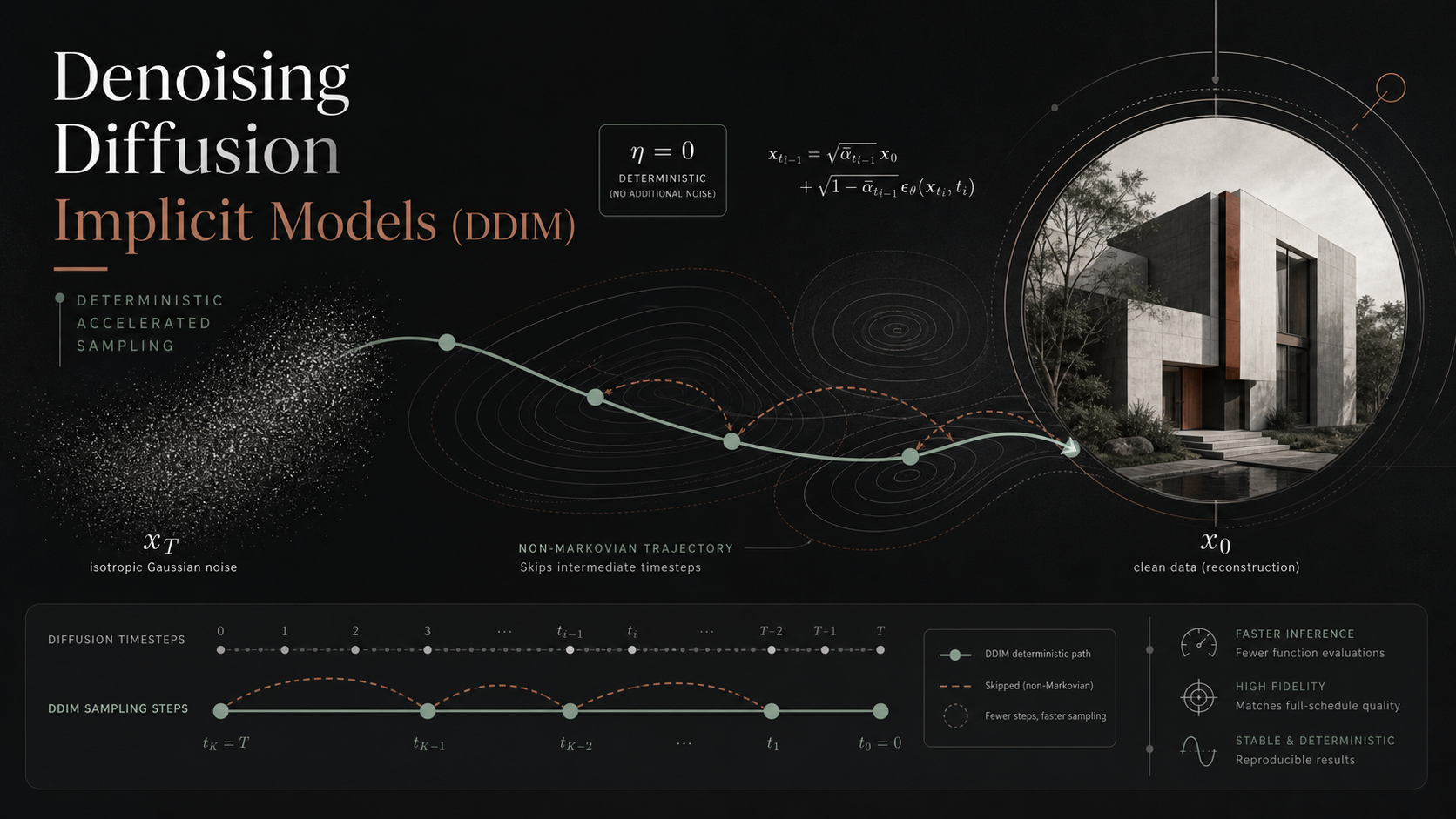
Denoising Diffusion Probabilistic Models (DDPMs) generate excellent images but require simulating a long Markov chain (often \(T=1000\) steps) to produce a single sample, because the generative process is defined as the reverse of a fixed Markovian forward diffusion. This paper observes that the training objective used by DDPMs only depends on the marginals \(q(x_t \mid x_0)\), not on the full joint forward process \(q(x_{1:T} \mid x_0)\). That means many different forward processes — including non-Markovian ones — share the same marginals and therefore the same (or an equivalent) training objective. The authors construct a family of non-Markovian forward processes indexed by a variance parameter \(\sigma\), derive a corresponding generative process for each, and show that a single DDPM checkpoint can be reused, without retraining, to sample from any member of this family. Setting \(\sigma = 0\) yields a fully deterministic generative process — the Denoising Diffusion Implicit Model (DDIM) — which can skip steps of the reverse chain, produce comparable or better samples in 10–50\(\times\) fewer steps, guarantees that the same initial noise \(x_T\) maps to visually consistent outputs across trajectories of different lengths, supports meaningful latent-space interpolation, and can be related to an ODE (an Euler discretization of a “probability flow” ODE), enabling near-exact encoding and reconstruction.
1. Motivation: Why DDPMs Are Slow
Deep generative models such as GANs, VAEs, autoregressive models, normalizing flows, and iterative denoising models (DDPMs, score-based models / NCSNs) all try to approximate a data distribution \(q(x_0)\) so that it is easy to sample from. GANs currently produce very sharp samples with a single forward pass through a generator network, but they are notoriously difficult to train (mode collapse, unstable optimization) and require careful architecture and hyperparameter choices.
DDPMs and Noise Conditional Score Networks (NCSNs) sidestep adversarial training entirely. They train a denoising autoencoder at many different noise levels and then produce a sample by iteratively denoising pure noise, using either Langevin-dynamics-like updates (NCSN) or the reverse of an explicit forward diffusion process (DDPM). This gets rid of adversarial instability, but the price is steep: because the generative Markov chain is the reverse of a forward chain with \(T\) steps (often \(T=1000\)), producing a single sample requires \(T\) sequential network evaluations. The paper quotes concrete numbers: roughly 20 hours to sample 50,000 images of size \(32\times32\) from a DDPM on an Nvidia 2080 Ti, versus under a minute for a GAN — and this gap balloons to roughly 1,000 hours for \(256\times256\) images. This makes DDPMs impractical wherever latency matters.
The central question the paper asks is: can we keep the same trained network and the same training objective, but design a much faster generative process?
2. Background: The DDPM Formalism
DDPMs are latent-variable models
\[p_{\theta}(x_0) = \int p_{\theta}(x_{0:T})\, dx_{1:T}, \qquad p_{\theta}(x_{0:T}) := p_{\theta}(x_T) \prod_{t=1}^{T} p_{\theta}^{(t)}(x_{t-1}\mid x_t) \tag{1}\]
where \(x_1, \dots, x_T\) live in the same space \(\mathcal{X}\) as \(x_0\). Training maximizes a variational lower bound on the log-likelihood:
\[\max_{\theta}\ \mathbb{E}_{q(x_0)}[\log p_\theta(x_0)] \;\le\; \max_\theta\ \mathbb{E}_{q(x_0,\dots,x_T)}\big[\log p_\theta(x_{0:T}) - \log q(x_{1:T}\mid x_0)\big] \tag{2}\]
Unlike a VAE, the inference distribution \(q(x_{1:T}\mid x_0)\) here is fixed, not learned. Ho et al. (2020) chose a Markov chain of Gaussian transitions parameterized by a decreasing sequence \(\alpha_{1:T} \in (0,1]^T\):
\[q(x_{1:T}\mid x_0) := \prod_{t=1}^T q(x_t \mid x_{t-1}), \quad q(x_t\mid x_{t-1}) := \mathcal{N}\!\Big(\sqrt{\tfrac{\alpha_t}{\alpha_{t-1}}}\, x_{t-1},\ \big(1 - \tfrac{\alpha_t}{\alpha_{t-1}}\big) I\Big) \tag{3}\]
This is called the forward process because it progressively injects noise as \(t\) increases from \(0\) to \(T\); the model \(p_\theta(x_{0:T})\) is the generative process because it progressively removes noise going from \(x_T\) back to \(x_0\) (this is exactly the picture in Figure 1, left panel, discussed below).
A crucial property of this construction is that the forward process has a simple closed form for jumping directly from \(x_0\) to any \(x_t\), without needing to simulate the intermediate steps:
\[q(x_t \mid x_0) = \mathcal{N}\big(x_t;\ \sqrt{\alpha_t}\, x_0,\ (1-\alpha_t) I\big) \tag{"special property"}\]
so we can write \(x_t\) as a noised version of \(x_0\):
\[x_t = \sqrt{\alpha_t}\, x_0 + \sqrt{1-\alpha_t}\,\epsilon, \qquad \epsilon \sim \mathcal{N}(0, I) \tag{4}\]
Choosing \(\alpha_T \approx 0\) makes \(q(x_T\mid x_0)\) converge to a standard Gaussian for every \(x_0\), motivating the prior \(p_\theta(x_T) := \mathcal{N}(0,I)\). If every conditional is Gaussian with a trainable mean and fixed variance, the ELBO in Eq. (2) simplifies to a weighted sum of denoising losses:
\[L_\gamma(\epsilon_\theta) := \sum_{t=1}^{T} \gamma_t\, \mathbb{E}_{x_0 \sim q(x_0),\, \epsilon_t \sim \mathcal{N}(0,I)}\Big[\big\|\epsilon_\theta^{(t)}(\sqrt{\alpha_t}x_0 + \sqrt{1-\alpha_t}\,\epsilon_t) - \epsilon_t\big\|_2^2\Big] \tag{5}\]
Here \(\epsilon_\theta = \{\epsilon_\theta^{(t)}\}_{t=1}^T\) is a (typically shared-parameter, time-conditioned) network that tries to predict the noise \(\epsilon_t\) that was added to produce \(x_t\). Ho et al. found that setting all weights \(\gamma_t = 1\) (rather than the theoretically-derived weights) produced the best samples in practice — this \(L_1\) objective is what the field commonly calls “the DDPM loss,” and it is the same objective used by score-matching-based NCSNs.
The key limitation: \(T\) is large (e.g., 1000) because a large \(T\) keeps each individual reverse transition close to Gaussian, which is required for the Gaussian parameterization of \(p_\theta^{(t)}\) to be a good approximation. But all \(T\) steps must be run sequentially to draw one sample — there’s no way to parallelize across \(t\).
3. The Key Idea: Non-Markovian Forward Processes with the Same Marginals
Look again at Eq. (5): the objective \(L_\gamma\) only involves the marginal distributions \(q(x_t\mid x_0)\) for each \(t\) — it never references the joint \(q(x_{1:T}\mid x_0)\) directly. This is the crux of the paper. Since infinitely many joint distributions can share the same set of marginals, the authors ask whether a non-Markovian joint could be constructed that (a) has the same marginals \(q(x_t\mid x_0) = \mathcal{N}(\sqrt{\alpha_t}x_0, (1-\alpha_t)I)\) for every \(t\), and (b) yields a generative process that is faster to sample from.
3.1 A family of non-Markovian inference processes
Consider a family \(\mathcal{Q}\) of inference distributions indexed by a vector \(\sigma \in \mathbb{R}^T_{\ge 0}\):
\[q_\sigma(x_{1:T}\mid x_0) := q_\sigma(x_T\mid x_0) \prod_{t=2}^{T} q_\sigma(x_{t-1}\mid x_t, x_0) \tag{6}\]
with \(q_\sigma(x_T\mid x_0) = \mathcal{N}(\sqrt{\alpha_T}x_0, (1-\alpha_T)I)\) and, for \(t>1\),
\[q_\sigma(x_{t-1}\mid x_t, x_0) = \mathcal{N}\!\left(\sqrt{\alpha_{t-1}}\,x_0 + \sqrt{1-\alpha_{t-1}-\sigma_t^2}\cdot \frac{x_t - \sqrt{\alpha_t}\,x_0}{\sqrt{1-\alpha_t}},\ \sigma_t^2 I\right) \tag{7}\]
The mean is chosen precisely so that, by induction (proved as Lemma 1 in the paper’s Appendix B and reproduced below), \(q_\sigma(x_t\mid x_0) = \mathcal{N}(\sqrt{\alpha_t}x_0, (1-\alpha_t)I)\) holds for every \(t\) — i.e., the marginals match the DDPM ones exactly, no matter what \(\sigma\) is. Applying Bayes’ rule gives the corresponding “forward” conditional
\[q_\sigma(x_t\mid x_{t-1}, x_0) = \frac{q_\sigma(x_{t-1}\mid x_t,x_0)\,q_\sigma(x_t\mid x_0)}{q_\sigma(x_{t-1}\mid x_0)} \tag{8}\]
which is also Gaussian, but now depends on both \(x_{t-1}\) and \(x_0\) rather than only on \(x_{t-1}\) — this is what makes the process non-Markovian. The magnitude of \(\sigma\) controls how stochastic this process is: as \(\sigma \to 0\), observing \(x_0\) and any single \(x_t\) pins down \(x_{t-1}\) almost exactly (it becomes near-deterministic).
Proof sketch of Lemma 1 (marginal matching by induction): Assume \(q_\sigma(x_t\mid x_0) = \mathcal{N}(\sqrt{\alpha_t}x_0, (1-\alpha_t)I)\) holds for some \(t\). Using the Gaussian marginalization identity \(q_\sigma(x_{t-1}\mid x_0) = \int q_\sigma(x_t\mid x_0)\, q_\sigma(x_{t-1}\mid x_t,x_0)\, dx_t\) and the standard formula for marginalizing a linear-Gaussian model (Bishop, PRML, Eq. 2.115), the resulting mean is
\[\mu_{t-1} = \sqrt{\alpha_{t-1}}\,x_0 + \sqrt{1-\alpha_{t-1}-\sigma_t^2}\cdot \frac{\sqrt{\alpha_t}x_0 - \sqrt{\alpha_t}x_0}{\sqrt{1-\alpha_t}} = \sqrt{\alpha_{t-1}}\, x_0\]
(the correction term vanishes because the two \(\sqrt{\alpha_t}x_0\) terms cancel), and the resulting covariance is
\[\Sigma_{t-1} = \sigma_t^2 I + \frac{1-\alpha_{t-1}-\sigma_t^2}{1-\alpha_t}(1-\alpha_t) I = (1-\alpha_{t-1}) I.\]
So \(q_\sigma(x_{t-1}\mid x_0) = \mathcal{N}(\sqrt{\alpha_{t-1}}x_0, (1-\alpha_{t-1})I)\), completing the induction (base case \(t=T\) holds by construction). \(\blacksquare\)
3.2 The matching generative process
Given a noisy \(x_t\), the natural strategy is: first predict what \(x_0\) probably was, then plug that prediction into \(q_\sigma(x_{t-1}\mid x_t, x_0)\) to sample \(x_{t-1}\). Concretely, since \(x_t = \sqrt{\alpha_t}x_0 + \sqrt{1-\alpha_t}\epsilon_t\) (Eq. 4), a network \(\epsilon_\theta^{(t)}(x_t)\) trained to predict the noise \(\epsilon_t\) gives us a denoised prediction of \(x_0\) for free:
\[f_\theta^{(t)}(x_t) := \big(x_t - \sqrt{1-\alpha_t}\cdot \epsilon_\theta^{(t)}(x_t)\big) / \sqrt{\alpha_t} \tag{9}\]
The generative process is then defined, with prior \(p_\theta(x_T) = \mathcal{N}(0,I)\), as
\[p_\theta^{(t)}(x_{t-1}\mid x_t) = \begin{cases}\mathcal{N}\big(f_\theta^{(1)}(x_1),\ \sigma_1^2 I\big) & t=1\\[4pt] q_\sigma\big(x_{t-1}\mid x_t,\, f_\theta^{(t)}(x_t)\big) & t>1\end{cases} \tag{10}\]
i.e., Eq. (7) with the true \(x_0\) replaced by the model’s prediction \(f_\theta^{(t)}(x_t)\). Training uses the variational objective
\[J_\sigma(\epsilon_\theta) := \mathbb{E}_{q_\sigma(x_{0:T})}\big[\log q_\sigma(x_{1:T}\mid x_0) - \log p_\theta(x_{0:T})\big] \tag{11}\]
At first glance it looks like a different model must be trained for every choice of \(\sigma\), since each \(\sigma\) defines a different objective \(J_\sigma\). The paper’s central theoretical result rules this out:
Theorem 1. For all \(\sigma > 0\), there exist \(\gamma \in \mathbb{R}^T_{>0}\) and \(C \in \mathbb{R}\) such that \(J_\sigma = L_\gamma + C\).
Proof (sketch). Expand \(J_\sigma\) and complete the square: each summand for \(t>1\) becomes a KL divergence between two Gaussians with the same variance \(\sigma_t^2\), which collapses to a squared-error term,
\[\mathbb{E}\big[D_{\mathrm{KL}}(q_\sigma(x_{t-1}\mid x_t,x_0)\,\|\,p_\theta^{(t)}(x_{t-1}\mid x_t))\big] = \mathbb{E}\left[\frac{\|x_0 - f_\theta^{(t)}(x_t)\|_2^2}{2\sigma_t^2}\right]\]
Substituting the definitions of \(x_0\) and \(f_\theta^{(t)}\) from Eq. (4) and (9), the \(x_t\)-dependent terms cancel and this reduces exactly to a rescaled noise-prediction error,
\[= \mathbb{E}_{x_0,\epsilon}\left[\frac{\|\epsilon - \epsilon_\theta^{(t)}(x_t)\|_2^2}{2 d\, \sigma_t^2 \alpha_t}\right]\]
where \(d = \dim(x_0)\). The \(t=1\) term reduces analogously. Hence, setting \(\gamma_t = 1/(2d\sigma_t^2\alpha_t)\) for every \(t\) gives \(J_\sigma(\epsilon_\theta) \equiv L_\gamma(\epsilon_\theta)\) for all \(\epsilon_\theta\), i.e., \(J_\sigma = L_\gamma + C\). \(\blacksquare\)
The payoff of Theorem 1 is enormous: since \(L_\gamma\)’s optimum does not depend on the weighting \(\gamma\) whenever parameters are not shared across timesteps (the global optimum is reached by independently minimizing each term of the sum), the \(L_1\)-trained DDPM network is already the optimal solution for every \(J_\sigma\). A single pretrained DDPM checkpoint can serve as the noise predictor for any member of this entire family of generative processes — no retraining required. The only thing that changes across family members is how you use the trained network at sampling time.
4. Sampling from Generalized Generative Processes
4.1 Denoising Diffusion Implicit Models (DDIM)
From Eq. (10), one can sample \(x_{t-1}\) from \(x_t\) via:
\[x_{t-1} = \sqrt{\alpha_{t-1}}\underbrace{\left(\frac{x_t - \sqrt{1-\alpha_t}\,\epsilon_\theta^{(t)}(x_t)}{\sqrt{\alpha_t}}\right)}_{\text{"predicted }x_0\text{"}} + \underbrace{\sqrt{1-\alpha_{t-1}-\sigma_t^2}\cdot \epsilon_\theta^{(t)}(x_t)}_{\text{"direction pointing to }x_t\text{"}} + \underbrace{\sigma_t \epsilon_t}_{\text{random noise}} \tag{12}\]
with \(\epsilon_t\sim\mathcal{N}(0,I)\) independent of \(x_t\), and \(\alpha_0 := 1\). Different choices of \(\sigma\) give different generative processes using the same \(\epsilon_\theta\):
- If \(\sigma_t = \sqrt{(1-\alpha_{t-1})/(1-\alpha_t)}\sqrt{1-\alpha_t/\alpha_{t-1}}\) for all \(t\), the forward process becomes Markovian again and the generative process reduces exactly to the original DDPM.
- If \(\sigma_t = 0\) for all \(t\), the forward process becomes deterministic given \(x_{t-1}\) and \(x_0\) (except at \(t=1\)), and the coefficient on the random noise term in Eq. (12) vanishes. The resulting model is an implicit probabilistic model — samples are a deterministic function of the initial latent \(x_T\). This is the Denoising Diffusion Implicit Model (DDIM), pronounced /ˈdɪm/, so named because it is an implicit model trained with the DDPM objective, even though its “forward process” is no longer a diffusion in the classical sense.
4.2 Accelerated Generation Processes (Sampling with Fewer Steps)
Because the denoising loss \(L_1\) never depended on the forward process having exactly \(T\) steps — only on the marginals \(q_\sigma(x_t\mid x_0)\) being fixed — we can define the forward process over just a subsequence \(\{x_{\tau_1}, \dots, x_{\tau_S}\}\), where \(\tau\) is an increasing subsequence of \([1,\dots,T]\) of length \(S \ll T\), while requiring \(q(x_{\tau_i}\mid x_0) = \mathcal{N}(\sqrt{\alpha_{\tau_i}}x_0, (1-\alpha_{\tau_i})I)\) to still match the marginals. The generative process then only needs to walk backwards along \(\tau\) — this reversed subsequence is called the sampling trajectory. Since sampling cost is linear in the number of steps taken, using \(S \ll T\) steps gives a proportional speedup.
Formally (Appendix C), the accelerated inference process factorizes as
\[q_{\sigma,\tau}(x_{1:T}\mid x_0) = q_{\sigma,\tau}(x_{\tau_S}\mid x_0)\prod_{i=1}^{S} q_{\sigma,\tau}(x_{\tau_{i-1}}\mid x_{\tau_i}, x_0) \prod_{t\in\bar\tau} q_{\sigma,\tau}(x_t\mid x_0) \tag{52}\]
where \(\bar\tau := \{1,\dots,T\}\setminus\tau\). Intuitively, \(\{x_{\tau_i}\}\) together with \(x_0\) form a chain (used to actually produce samples), while the remaining \(\{x_t\}_{t\in\bar\tau}\) together with \(x_0\) form a star graph (only needed to keep the variational bound well-defined — see Figure 2 below). A similar argument to Theorem 1’s proof shows this accelerated objective is also equivalent (up to reweighting) to \(L_\gamma\), so — again — no retraining is required; only the sampling procedure changes.
Two practical choices for picking the subsequence \(\tau\) (Appendix D.2) are used in the experiments: linear (\(\tau_i = \lfloor ci\rfloor\)) and quadratic (\(\tau_i=\lfloor ci^2\rfloor\)) spacing, with \(c\) chosen so \(\tau_S \approx T\). The paper uses quadratic spacing for CIFAR-10 and linear spacing for the other datasets, each found empirically to give marginally better FID than the alternative.
4.3 Connection to Neural ODEs
Rewriting the DDIM update (Eq. 12, with \(\sigma_t=0\)) in terms of a small step \(\Delta t\) reveals a resemblance to an Euler discretization of an ODE:
\[\frac{x_{t-\Delta t}}{\sqrt{\alpha_{t-\Delta t}}} = \frac{x_t}{\sqrt{\alpha_t}} + \left(\sqrt{\frac{1-\alpha_{t-\Delta t}}{\alpha_{t-\Delta t}}} - \sqrt{\frac{1-\alpha_t}{\alpha_t}}\right)\epsilon_\theta^{(t)}(x_t) \tag{13}\]
Reparameterizing with \(\bar x := x/\sqrt{\alpha}\) and \(\sigma(t) := \sqrt{(1-\alpha(t))/\alpha(t)}\) (an increasing, continuous function with \(\sigma(0)=0\)), taking \(\Delta t \to 0\) turns Eq. (13) into the ODE
\[d\bar x(t) = \epsilon_\theta^{(t)}\!\left(\frac{\bar x(t)}{\sqrt{\sigma^2(t)+1}}\right) d\sigma(t) \tag{14}\]
with initial condition \(\bar x(T) \sim \mathcal{N}(0,\sigma(T)^2 I)\) for large \(\sigma(T)\). Because this is an ODE (not an SDE), it can, with a fine enough discretization, be simulated forward in time (\(t=0\to T\), encoding \(x_0\to x_T\)) just as easily as backward (\(t=T\to0\), generating \(x_0\) from \(x_T\)). This is a property DDPMs fundamentally lack, since their reverse process is stochastic.
Proposition 1. The ODE in Eq. (14), evaluated at the optimal \(\epsilon_\theta^{(t)}\), is equivalent to the probability-flow ODE corresponding to the “Variance-Exploding” (VE) SDE of Song et al. (2020) — a continuous-time generalization of NCSN-style score-based models.
Proof idea. Reparameterize with \(\bar x(t) = \bar x(0) + \sigma(t)\epsilon\), matching the VE-SDE convention. The DDIM-derived ODE (Eq. 45 in the appendix) is \(\frac{d\bar x}{dt} = \frac{d\sigma}{dt}\,\epsilon_\theta^{(t)}\big(\bar x/\sqrt{\sigma^2+1}\big)\). Independently, the probability-flow ODE for a VE-SDE is \(d\bar x = -\tfrac12 g(t)^2 \nabla_{\bar x}\log p_t(\bar x)\, dt\) with \(g(t)^2 = d\sigma^2(t)/dt\). Using the fact that the optimal noise predictor and the optimal score function are related by \(\nabla_{\bar x}\log p_t(\bar x) = -\epsilon_\theta^{(t)}(\bar x/\sqrt{\sigma^2+1})/\sigma(t)\) (a standard denoising-score-matching identity), substituting into the probability-flow ODE and simplifying recovers exactly \(\frac{d\bar x}{dt} = \frac{d\sigma}{dt}\epsilon_\theta^{(t)}(\cdot)\) — identical to the DDIM ODE. \(\blacksquare\)
Although the two ODEs are mathematically identical, their discretizations differ: DDIM’s Euler steps are taken with respect to \(\sigma(t)\), while the probability-flow ODE’s Euler steps (Eq. 15 in the paper) are taken with respect to \(t\) directly. These coincide when \(\alpha_t\) and \(\alpha_{t-\Delta t}\) are close, but diverge for large steps — which is precisely the regime accelerated sampling operates in, explaining why the two integration schemes behave differently at low step counts in practice.
5. Algorithms
The paper does not present its methods as boxed pseudocode, but the two procedures below (training, and generalized sampling) directly formalize Eq. (5) and Eq. (12)/(52), and match how DDIM is implemented in practice.
Algorithm 1 — Training (unchanged from DDPM)
Input: data distribution q(x0), noise schedule alpha_1..alpha_T, network eps_theta
repeat
    sample x0 ~ q(x0)
    sample t ~ Uniform({1, ..., T})
    sample epsilon ~ N(0, I)
    x_t = sqrt(alpha_t) * x0 + sqrt(1 - alpha_t) * epsilon
    take gradient step on
        grad_theta || epsilon - eps_theta(x_t, t) ||^2
until converged
Algorithm 2 — Generalized (DDIM/DDPM) Sampling
Input: trained eps_theta, schedule alpha_1..alpha_T, sub-sequence tau = [tau_1 < ... < tau_S = T],
       stochasticity coefficients sigma_{tau_i} (sigma = 0 gives DDIM; a specific sigma_t gives DDPM)
x_{tau_S} ~ N(0, I)
for i = S, S-1, ..., 1:
    predict noise:      eps_hat = eps_theta(x_{tau_i}, tau_i)
    predict x0:          x0_hat = (x_{tau_i} - sqrt(1 - alpha_{tau_i}) * eps_hat) / sqrt(alpha_{tau_i})
    direction to x_t:     dir    = sqrt(1 - alpha_{tau_{i-1}} - sigma_{tau_i}^2) * eps_hat
    sample noise:         z ~ N(0, I)  if i > 1 else z = 0
    x_{tau_{i-1}} = sqrt(alpha_{tau_{i-1}}) * x0_hat + dir + sigma_{tau_i} * z
return x_{tau_0}  # = x0
Setting \(\sigma \equiv 0\) for every step removes the stochastic term entirely, giving deterministic DDIM sampling; setting \(\dim(\tau) = T\) (i.e. \(\tau = [1,\dots,T]\)) with the DDPM-matching \(\sigma_t\) recovers the original full-length DDPM sampler. Everything in between — fewer steps, partial stochasticity via \(\eta\) (Section 6 below) — is available immediately, from the same checkpoint.
6. Experiments
All experiments reuse a single trained model per dataset (\(T=1000\), trained with the \(L_1\) objective from Eq. 5, exactly as in Ho et al. 2020) — datasets are CIFAR-10 (\(32\times32\)), CelebA (\(64\times64\)), LSUN Bedroom, and LSUN Church (both \(256\times256\)). Only the sampling procedure changes across experiments, controlled by two knobs: the sub-sequence \(\tau\) (how many/which steps to use) and a stochasticity interpolation parameter \(\eta\), defined so that
\[\sigma_{\tau_i}(\eta) = \eta\sqrt{\frac{1-\alpha_{\tau_{i-1}}}{1-\alpha_{\tau_i}}}\sqrt{1-\frac{\alpha_{\tau_i}}{\alpha_{\tau_{i-1}}}} \tag{16}\]
\(\eta=0\) recovers DDIM (fully deterministic); \(\eta=1\) recovers the original DDPM. The paper also benchmarks \(\hat\sigma\), a larger-variance DDPM variant used by Ho et al. (2020) specifically for their CIFAR-10 results.
6.1 Sample Quality vs. Efficiency
Measuring Fréchet Inception Distance (FID; lower is better) while varying the number of sampling steps \(\dim(\tau) \in \{10,20,50,100,1000\}\):
| \(\eta\) | CIFAR-10 S=10 | S=20 | S=50 | S=100 | S=1000 | CelebA S=10 | S=20 | S=50 | S=100 | S=1000 |
|---|---|---|---|---|---|---|---|---|---|---|
| 0.0 (DDIM) | 13.36 | 6.84 | 4.67 | 4.16 | 4.04 | 17.33 | 13.73 | 9.17 | 6.53 | 3.51 |
| 0.2 | 14.04 | 7.11 | 4.77 | 4.25 | 4.09 | 17.66 | 14.11 | 9.51 | 6.79 | 3.64 |
| 0.5 | 16.66 | 8.35 | 5.25 | 4.46 | 4.29 | 19.86 | 16.06 | 11.01 | 8.09 | 4.28 |
| 1.0 (DDPM) | 41.07 | 18.36 | 8.01 | 5.78 | 4.73 | 33.12 | 26.03 | 18.48 | 13.93 | 5.98 |
| \(\hat\sigma\) | 367.43 | 133.37 | 32.72 | 9.99 | 3.17 | 299.71 | 183.83 | 71.71 | 45.20 | 3.26 |
Similarly, on the larger LSUN datasets:
| Bedroom S=10 | S=20 | S=50 | S=100 | Church S=10 | S=20 | S=50 | S=100 | |
|---|---|---|---|---|---|---|---|---|
| DDIM (\(\eta=0\)) | 16.95 | 8.89 | 6.75 | 6.62 | 19.45 | 12.47 | 10.84 | 10.58 |
| DDPM (\(\eta=1\)) | 42.78 | 22.77 | 10.81 | 6.81 | 51.56 | 23.37 | 11.16 | 8.27 |
(For reference, the 1000-step DDPM baseline FIDs are 6.36 for Bedroom and 7.89 for Church.)
Takeaways: as \(\dim(\tau)\) grows, quality improves for every method (expected trade-off between compute and quality). DDIM (\(\eta=0\)) is consistently the best or tied-best at every step count, and its advantage is largest exactly where it matters most — few steps. DDPM-style stochastic sampling (\(\eta=1\), \(\hat\sigma\)) degrades sharply as \(\dim(\tau)\) shrinks; \(\hat\sigma\) in particular becomes extremely poor at low step counts because FID is highly sensitive to the added noisy perturbations it introduces. Wall-clock time scales linearly with the number of sampling steps (Figure 4 in the paper), so DDIM’s ability to hit “1000-step quality” using only 20–100 steps translates directly into a \(10\times\)–\(50\times\) real speedup; e.g., the 100-step DDPM on CelebA is roughly matched in FID by the 20-step DDIM.
6.2 Sample Consistency
Because DDIM’s generative process is a deterministic function of \(x_T\), fixing \(x_T\) and varying the sampling trajectory \(\tau\) (i.e., varying how many/which intermediate steps are taken) produces images that share the same high-level content, with only fine details varying. Even a 20-step trajectory already captures most of the high-level structure that a 1000-step trajectory would produce. This strongly suggests that \(x_T\) alone functions as a semantically meaningful latent code — an unusual property for a diffusion-style model, and one that DDPM’s stochastic sampling cannot offer (identical \(x_T\) under DDPM yields highly diverse outputs).
6.3 Latent-Space Interpolation
Since high-level content is encoded in \(x_T\), the authors test whether interpolating in the latent space, as is common for GANs, produces meaningful interpolation in image space. Two random \(x_T^{(0)}, x_T^{(1)} \sim \mathcal{N}(0,I)\) are combined with spherical linear interpolation (slerp), which is the natural way to interpolate points that are meant to lie roughly on a Gaussian’s typical “shell”:
\[x_T^{(\alpha)} = \frac{\sin((1-\alpha)\theta)}{\sin\theta}\, x_T^{(0)} + \frac{\sin(\alpha\theta)}{\sin\theta}\, x_T^{(1)}, \qquad \theta = \arccos\!\left(\frac{x_T^{(0)\top}x_T^{(1)}}{\|x_T^{(0)}\|\,\|x_T^{(1)}\|}\right) \tag{67}\]
Each interpolated \(x_T^{(\alpha)}\) is then decoded with DDIM. The resulting sequences show smooth, semantically coherent transitions (pose, identity, background attributes blending gradually) — a property DDPM cannot replicate directly, since re-using the same \(x_T\) under DDPM’s stochastic decoder does not pin down a consistent \(x_0\).
6.4 Reconstruction from Latent Space
Because DDIM corresponds to an ODE, it should be approximately invertible: encode \(x_0\to x_T\) by simulating Eq. (14) forward, then decode \(x_T\to x_0\) by simulating it backward, and measure the reconstruction error.
| \(S\) (steps) | 10 | 20 | 50 | 100 | 200 | 500 | 1000 |
|---|---|---|---|---|---|---|---|
| Per-dim MSE | 0.014 | 0.0065 | 0.0023 | 0.0009 | 0.0004 | 0.0001 | 0.0001 |
Reconstruction error shrinks steadily and monotonically as the number of discretization steps \(S\) increases — exactly the behavior expected of an Euler-integrated ODE as its step size shrinks, and analogous to what invertible flows / Neural ODEs exhibit. DDPMs, being fundamentally stochastic in their generative process, cannot do this at all.
8. Discussion, Limitations, and Future Directions
The paper closes by noting that the non-Markovian construction opens the door to forward processes that are not Gaussian at all — something the original diffusion framework could not do, since Gaussian is the unique stable distribution with finite variance. As a proof of concept, Appendix A works out an analogous non-Markovian construction for discrete/categorical data (see below). The authors also flag the ODE connection as an especially promising direction: numerical methods that reduce discretization error beyond simple Euler steps — e.g., multistep methods like Adams–Bashforth — could plausibly improve sample quality at a fixed, small step budget, since DDIM sampling is mathematically just Euler integration of an ODE. This idea would later be highly influential in the diffusion literature (fast ODE/SDE solvers, DPM-Solver, and related accelerated samplers, are direct intellectual descendants of this observation, though they postdate this paper).
Appendix A: The discrete/categorical case (briefly)
For a one-hot categorical \(x_0\) with \(K\) classes, define \(q(x_t\mid x_0) = \mathrm{Cat}(\alpha_t x_0 + (1-\alpha_t)\mathbf{1}_K)\) (a mixture that gradually forgets the true class in favor of the uniform distribution \(\mathbf{1}_K/K\)). An analogous non-Markovian \(q(x_{t-1}\mid x_t,x_0)\) is defined as a three-way mixture over “keep \(x_t\)”, “reveal \(x_0\)”, and “go fully uniform,” with mixture weights chosen so the marginals match. The KL divergence between this and the model’s own reverse conditional \(p_\theta(x_{t-1}\mid x_t)\) reduces to (an upper bound of) a standard multi-class classification loss, mirroring the Gaussian case’s reduction to squared error. The authors leave a full empirical study of this discrete variant to future work, but note it suggests DDIM-style acceleration is not intrinsically tied to continuous, Gaussian diffusions.
9. Diagrams
The paper contains two genuinely conceptual (graph-structure) figures; the remaining figures (3–10) are qualitative sample grids or scalar performance plots rather than structural diagrams, so they are summarized in prose above (Sections 6.1–6.4) instead of being redrawn here.
Figure 1 — Graphical models: Markovian diffusion (left) vs. non-Markovian inference (right)
In the original DDPM, each \(x_t\) is generated only from \(x_{t-1}\) (a first-order Markov chain), and the reverse/generative process retraces the same chain backward. In the non-Markovian family the paper introduces, every \(x_{t-1}\) is conditioned jointly on both \(x_t\) and \(x_0\) — shown by the extra arrows from \(x_0\) fanning out to every latent variable.
graph LR
  subgraph "Markovian diffusion (DDPM)"
    direction LR
    A0["x0"] --> A1["x1"] --> A2["x2"] --> Adots["..."] --> AT["xT"]
    AT -.generative process.-> Adots -.-> A2 -.-> A1 -.-> A0
  end
graph LR
  subgraph "Non-Markovian inference (DDIM family)"
    direction LR
    B0["x0"] --> B1["x1"]
    B0 --> B2["x2"]
    B0 --> Bdots["..."]
    B0 --> BT["xT"]
    B1 --> B2
    B2 --> Bdots
    Bdots --> BT
    BT -.generative process.-> Bdots
    Bdots -.-> B2
    B2 -.-> B1
    B1 -.-> B0
  end
Reading the diagrams: solid arrows denote the (non-)Markovian forward/inference dependencies; dashed arrows denote the direction the trained generative process actually samples in (from \(x_T\) down to \(x_0\)). In the right-hand diagram, note that \(x_0\) has a direct edge into every \(x_t\) — this is exactly the extra conditioning that makes the process non-Markovian, and it is what allows the reverse chain to legally “jump” over intermediate steps (Figure 2, next).
Figure 2 — Accelerated generation with \(\tau = [1, 3]\)
When sampling is accelerated, the generative process only visits a subsequence \(\tau\) of the original \(T\) timesteps (here, as a minimal illustrative example with \(T=3\), only \(x_1\) and \(x_3=x_T\) are visited; \(x_2\) is skipped entirely at sampling time, existing only conceptually as part of keeping the variational bound consistent).
graph LR
  subgraph "Accelerated sampling trajectory, tau = [1, 3]"
    direction LR
    X0["x0"] --> X1["x1 (tau_1, sampled)"]
    X0 --> X2["x2 (skipped at sampling time)"]
    X0 --> X3["x3 = xT (tau_2, sampled)"]
    X1 --> X3
    X3 -.DDIM step.-> X1
    X1 -.DDIM step.-> X0
  end
Reading the diagram: the solid edges from \(x_0\) show which latents remain tied to \(x_0\)’s marginal constraint; the edge \(x_1 \to x_3\) (and its dashed reverse) is the direct jump the accelerated sampler takes — going straight from \(x_3\) to \(x_1\), then from \(x_1\) to \(x_0\), entirely skipping \(x_2\). This is the mechanism, generalized to \(S \ll T\) chosen steps out of \(T\), that gives DDIM its \(10\times\)–\(50\times\) wall-clock speedup.
10. Key Takeaways
The central theoretical contribution is deceptively simple but far-reaching: the DDPM training objective is a property of marginals, not of any particular Markov chain, so a whole family of non-Markovian generative processes — parameterized by a stochasticity knob \(\sigma\) (or, in the experiments, \(\eta\)) and a sampling-trajectory length \(S\) — can all be driven by exactly the same trained noise-prediction network. Setting stochasticity to zero yields DDIM, a deterministic implicit model that (a) samples 10–50\(\times\) faster than DDPM at comparable or better quality, (b) produces trajectory-length-consistent outputs from a fixed latent, (c) supports meaningful latent interpolation via slerp, and (d) is exactly the Euler discretization of a probability-flow ODE, enabling near-lossless encode/decode. These properties collectively foreshadow much of the later fast-sampler and ODE/SDE-solver literature for diffusion models.