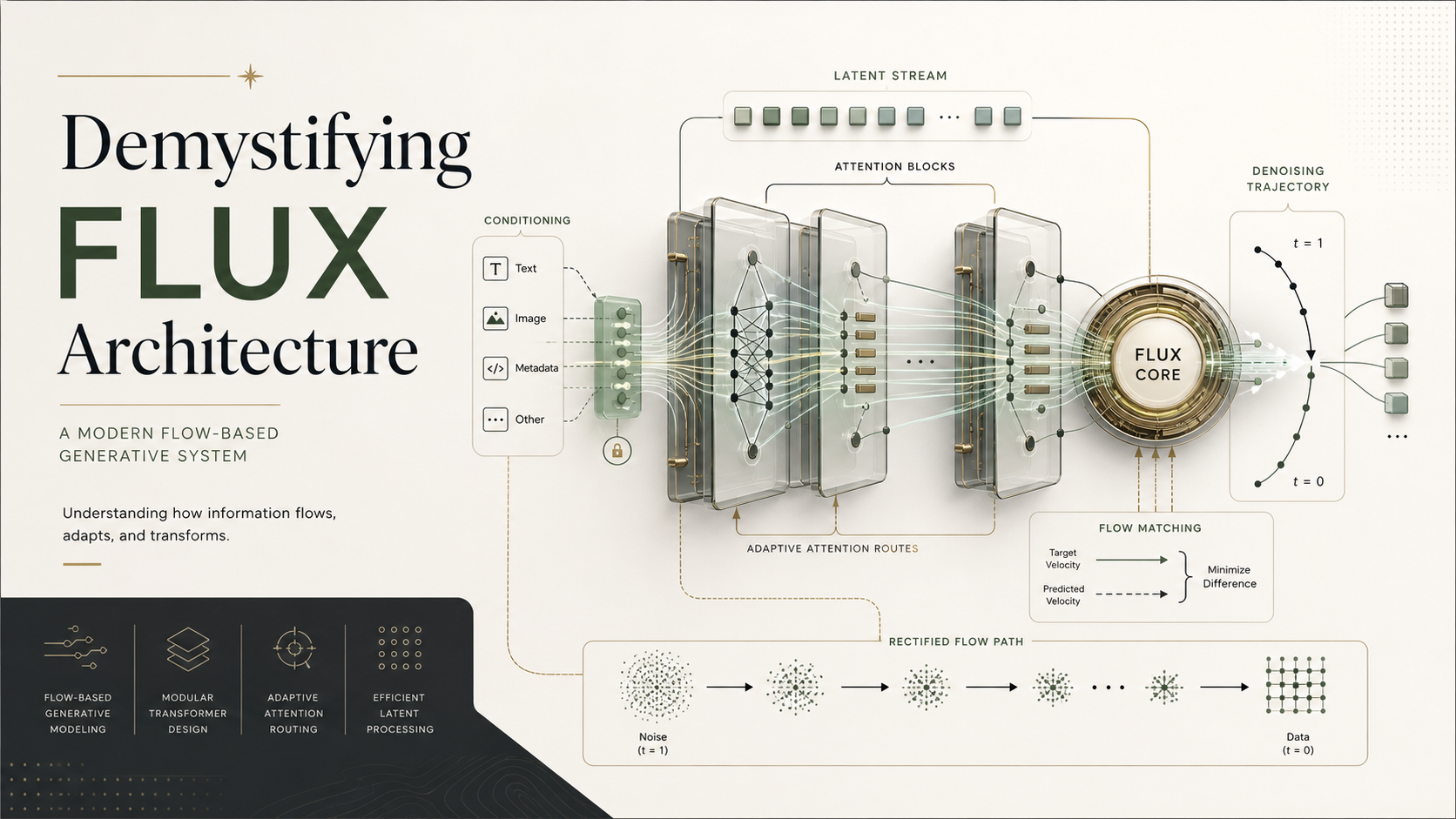
This is an unofficial reader’s guide reformatting the reverse-engineering report “Demystifying Flux Architecture” (arXiv:2507.09595, submitted 13 Jul 2025, CC BY 4.0). All architecture diagrams from the original paper have been redrawn as Mermaid flowcharts for native rendering and version control. Photographic and bar-chart figures (qualitative image comparisons, ELO score plots) are summarized in prose instead, since they don’t encode a process or architecture a flowchart could represent. Each diagram is annotated with the source figure number it reinterprets, for traceability back to the original PDF/HTML.
This report is not published or endorsed by Black Forest Labs.
Abstract
FLUX.1 is a diffusion-based text-to-image generation model developed by Black Forest Labs, designed to achieve faithful text-image alignment while maintaining high image quality and diversity. FLUX is considered state-of-the-art in text-to-image generation, outperforming popular models such as Midjourney, DALL·E 3, Stable Diffusion 3 (SD3), and SDXL. Although publicly available as open source, the authors have not released official technical documentation detailing the model’s architecture or training setup. This report summarizes an extensive reverse-engineering effort aimed at demystifying FLUX’s architecture directly from its source code, to support its adoption as a backbone for future research and development.
Background
To understand FLUX’s design choices, it helps to walk through the lineage of models and methods that shaped it: generative modeling broadly, diffusion models specifically, Stable Diffusion’s evolution, Rectified Flow as a training paradigm, and the Transformer architecture that FLUX adopts as its full backbone.
ML-Based Image Generation
Image generation, in the machine-learning sense, means learning to sample novel images from a distribution that mimics some source dataset. A common strategy is to learn a mapping from the complex data distribution (natural images) to something simple and easy to sample from, typically an isotropic Gaussian — and then invert that mapping at generation time.
Several major families implement this idea:
- Variational Autoencoders (VAEs) — learn an encoder/decoder pair with a regularized latent space.
- Generative Adversarial Networks (GANs) — pit a generator against a discriminator in an adversarial game.
- Normalizing Flows (NFs) — learn an invertible, exact-likelihood transformation between data and noise.
- Diffusion Models (DMs) — learn to reverse a gradual noising process.
Among these families, text-to-image models — DALL·E, Stable Diffusion, and FLUX among them — have become the dominant paradigm for producing high-quality images from natural-language prompts.
Diffusion Models
Diffusion Models (DMs) are today’s state-of-the-art approach for text-conditioned image generation. Training corrupts clean images with Gaussian noise according to a timestep-dependent schedule, and the network learns to undo that corruption. Early diffusion models used U-Net backbones — convolutional layers augmented with attention for image–text alignment — but newer models such as SD3 and FLUX.1 have moved to fully Transformer-based denoisers, trading convolutional inductive bias for scalability and better long-range context modeling.
In the most common formulation, the network is trained to predict the (normalized) noise \(\epsilon\) that was added to a clean sample, using a simple reconstruction loss:
\[ \mathcal{L}_{\epsilon} = \mathbb{E}_{x_t, \epsilon, t}\Big[\|\epsilon_\theta(x_t, t) - \epsilon\|^2\Big] \tag{1}\]
where the noisy sample at timestep \(t\) is
\[ x_t = \sqrt{\alpha_t}\, x + \sqrt{1-\alpha_t}\, \epsilon,\qquad \epsilon \sim \mathcal{N}(0,1) \]
and \(x_0\) denotes the clean image. At inference time, the model starts from pure Gaussian noise and iteratively denoises it into a realistic image (Equation 1). Compared to GANs’ adversarial objective, this reconstruction-based training is more stable and scales better to high resolutions, while also enabling fine-grained control for tasks like super-resolution, inpainting, and text-conditioned synthesis.
Stable Diffusion
Stable Diffusion is a family of Latent Diffusion Models (LDMs): rather than diffusing directly in pixel space, images are first compressed into a lower-dimensional latent space by a pretrained autoencoder, the diffusion process runs in that latent space, and a decoder maps the final latent back to pixels. This dramatically reduces compute cost while preserving visual fidelity.
The lineage, as covered in the paper:
- SD 1.x (1.0–1.5): frozen CLIP text encoder + U-Net latent denoiser, trained on LAION-2B subsets. Open-source release drove rapid adoption and fine-tuning.
- SD 2.1: switched to OpenCLIP, trained at higher resolution (768×768), improving structure and fidelity.
- SDXL: two-stage base + refiner architecture, better handling of complex prompts, closer to commercial-grade realism.
- SD-Turbo: near real-time generation via Adversarial Diffusion Distillation (ADD) — a student model distilled from a teacher (SD2.1 or SDXL) to require far fewer steps.
- SD3: adopts a diffusion-transformer backbone and multimodal training, integrating text and image understanding jointly — a direct architectural precursor to FLUX (see Section 3.3).
Rectified Flows
Rectified Flow (RF) is the training paradigm FLUX actually uses instead of standard DM noise-prediction. It’s a training scheme, not an architectural change, but it matters here because it shapes what the FLUX transformer is trained to predict. RF builds on the Flow Matching framework and replaces stochastic denoising with a deterministic vector field.
Standard diffusion models train \(\epsilon_\theta\) to predict the noise added to a sample (Equation 1). Rectified Flow instead trains a model \(v_\theta\) to predict the velocity — a vector pointing from a noise sample toward a data sample along a straight interpolation path:
\[ \mathcal{L}_v = \mathbb{E}_{x_0, x_1, t}\Big[\|v_\theta(x_t, t) - (x_1 - x_0)\|^2\Big] \tag{2}\]
where
\[ x_t = (1-t)\,x_0 + t\,x_1,\qquad x_0 \sim \mathcal{N}(0, I),\quad x_1 \sim p_{\text{data}} \]
In Rectified Flow (Equation 2), \(x_0\) denotes noise and \(x_1\) denotes the data point — the opposite of standard DM convention, where \(x_0\) is the clean image. This flip resurfaces later in FLUX’s own sampling notation (Section 3.2), so keep it in mind when comparing equations across sections.
By defining a deterministic transport path from noise to data, RF avoids explicit noise schedules and stochastic sampling, solving instead a simple ODE with a learned velocity field — generally faster and more stable to train and sample from than classic diffusion.
Transformers
Transformers, originally built for NLP, introduced the self-attention mechanism: a way for every element of a sequence to weigh its relationship to every other element. This has become the substrate for state-of-the-art models across text, image, video, and multimodal domains.
Each attention block projects the input embeddings into query (\(Q\)), key (\(K\)), and value (\(V\)) matrices via learned linear layers, then computes:
\[ \text{Attention}(Q, K, V) = \text{softmax}\!\left(\frac{QK^{T}}{\sqrt{d_k}}\right)\cdot V \tag{3}\]
where \(d_k\) is the key dimensionality and the softmax normalizes attention weights to sum to 1 (Equation 3). In practice, multi-head attention runs several \(Q\)/\(K\)/\(V\) projections in parallel so the model can capture different types of relationships simultaneously.
For vision, Vision Transformers (ViTs) tokenize an image into fixed-size, non-overlapping patches (e.g., 16×16 pixels), flatten and linearly project each patch, then feed the resulting sequence — with positional encodings added — through a standard transformer encoder. This lets ViTs model long-range dependencies without a convolutional inductive bias.
Two attention regimes matter for what follows:
- Self-Attention: \(Q\), \(K\), and \(V\) are all projected from the same input embedding.
- Cross-Attention: used in text-to-image generation to condition image synthesis on a prompt — \(Q\) comes from image tokens, while \(K\) and \(V\) come from text embeddings.
FLUX, as we’ll see, uses a joint scheme that blends both ideas: a Multi-Modal Attention where text and image tokens are concatenated and attend to each other simultaneously.
FLUX.1
Introduction
FLUX.1 is a rectified-flow transformer trained in the latent space of an image autoencoder, released by Black Forest Labs in August 2024. The FLUX.1 family sets a new state-of-the-art for text-to-image tasks on both output quality and image–text alignment, as measured by ELO-score human-preference comparisons against Midjourney, DALL·E 3, SD3, and others across dimensions like prompt following, size/aspect variability, typography, output diversity, and visual quality. These ELO comparisons are bar-chart evaluations reproduced from the official Black Forest Labs announcement — not architecture diagrams — so they are summarized here in prose rather than redrawn.
While Black Forest Labs states FLUX follows the Rectified Flow training paradigm, the actual training setup — dataset, noise/timestep scheduling, hyperparameters — has never been publicly disclosed. What can be reverse-engineered is the model’s architecture and inference-time behavior, directly from the public inference code (the diffusers implementation). That’s the paper’s core contribution, and this guide follows the same top-down path: first a bird’s-eye view of the architecture, then the sampling pipeline, then a deep dive into the transformer itself.
flowchart LR
    P["Text Prompt"] --> TE["Text Encoders (CLIP + T5)"]
    TE --> EMB["Text Embeddings"]
    N["Gaussian Noise z0"] --> LAT["Latent Image Tokens"]
    EMB --> TB["FLUX Transformer Blocks (Double-Stream + Single-Stream)"]
    LAT --> TB
    TB -->|"repeat across sampling timesteps"| TB
    TB --> DEC["Pretrained VAE Decoder"]
    DEC --> IMG["Generated RGB Image"]
Figure 1 gives the top-level view: iterative refinement of latent + text tokens through transformer blocks, followed by VAE decoding.
FLUX.1 Sampling Pipeline
For simplicity, the paper (and this guide) describes sampling conditioned on a single prompt at a time. Like LDM, FLUX operates in a latent space: the final latent is decoded back into an RGB image. Following LDM’s approach, Black Forest Labs trained a convolutional autoencoder from scratch with an adversarial objective, but scaled the latent channel count from 4 (LDM) up to 16.
The sampling pipeline has three phases:
- Initiation and Pre-processing
- Iterative Refinement
- Post-processing
The notation follows the official diffusers implementation of the FLUX.1 pipeline.
Initiation and Pre-processing
The pipeline takes four required inputs:
- text — the textual prompt guiding generation.
- guidance_scale — controls conditioning strength.
- num_inference_steps — number of iterative sampling steps.
- resolution — spatial (height × width) resolution of the output image.
flowchart TD
    subgraph INIT["Initiation and Pre-processing"]
        TXT["text"] --> T5["T5 Encoder"]
        T5 --> EHS["encoder_hidden_states (dense, per-token)"]
        TXT --> CLIP["CLIP Encoder"]
        CLIP --> PP["pooled_projection (single vector)"]
        NIS["num_inference_steps"] --> TS["timestep subset, t in 0..T, T approx 1000"]
        RES["resolution H,W"] --> LATSHAPE["latent shape h,w = H,W // VAE_scale(8)"]
        LATSHAPE --> Z0["z0 ~ N(0,1)"]
        LATSHAPE --> IDS["img_ids per token; text_ids = n*(0,0,0)"]
        GS["guidance_scale"] --> GU["guidance"]
    end

    subgraph ITER["Iterative Refinement"]
        LOOP["for t in timesteps: z_(t+dt) = Samp(v_theta(z_t, t, Phi))"]
    end

    EHS --> LOOP
    PP --> LOOP
    GU --> LOOP
    Z0 --> LOOP
    IDS --> LOOP
    TS --> LOOP
    LOOP -->|"iterate t: 0 to 1"| LOOP
    LOOP --> Z1["z1 (clean latent)"]

    subgraph POST["Post-processing"]
        Z1 --> VAE["Pretrained VAE Decoder"]
        VAE --> IMG["RGB Image x1"]
    end
Each input is preprocessed as follows (see Figure 2):
- text is encoded by two pretrained text encoders:
- T5 produces dense, per-token embeddings — the
encoder_hidden_states. - CLIP produces a single pooled embedding for the whole prompt (like a CLS token) — the
pooled_projection.
- T5 produces dense, per-token embeddings — the
- num_inference_steps determines how many timesteps are sampled from the full diffusion range \(t \in [0:T]\), typically \(T = 1000\). These selected timesteps define the sampling trajectory.
- resolution determines the spatial shape of the initial latent noise \(z_0 \sim \mathcal{N}(0,1)\). Given target pixel resolution \((H, W)\), the latent dimensions are \((h = H\,/\!/\,\text{VAE}_{scale},\ w = W\,/\!/\,\text{VAE}_{scale})\) with \(\text{VAE}_{scale} = 8\). The image-token grid is further downsampled to \((h\,/\!/\,2,\ w\,/\!/\,2)\), and each token gets a unique identifier \((t, \hat h, \hat w)\) locating it on a 2D grid — these are the
img_ids. Thetext_idsreuse the same structure but with \(t = \hat h = \hat w = 0\) for every one of the \(n = 512\) (T5’s max token count) text tokens:text_ids = n·(0,0,0).
Iterative Refinement and Post-processing
Let \(\Phi = [\text{encoder\_hidden\_states}, \text{pooled\_projection}, \text{guidance}, \text{img\_ids}, \text{text\_ids}]\) denote the set of preprocessed, constant inputs. As in standard diffusion sampling, \([z_t, t, \Phi]\) is fed into the transformer at every sampling iteration:
\[ \forall\, t \in \text{timesteps}:\quad z_{t+\Delta t} = \text{Samp}\big(v_\theta(z_t, t, \Phi)\big) \tag{4}\]
where \(v_\theta\) is the network estimating the velocity vector (Section 2.4), and \(\text{Samp}(\cdot)\) is the Flow-Matching Euler Discrete sampler.
In Equation 4, timesteps runs from \(0\) to \(1\), with \(z_1\) the clean image latent and \(z_0\) pure Gaussian noise — the reverse of typical DM convention (compare with Equation 1 where \(x_0\) is clean). Don’t conflate FLUX’s sampling-time \(z_0\)/\(z_1\) with the RF training notation in Equation 2.
After the iterative refinement finishes, the final clean latent \(z_1\) is decoded by the pretrained VAE into the final image \(x_1\).
Transformer
The core of FLUX.1’s pipeline is the velocity predictor \(v_\theta\), optimized to estimate the velocity vector along the sampling trajectory. Like SD3, FLUX.1 replaces the conventional U-Net with a fully transformer-based design.
On every sampling iteration, inputs are preprocessed, then passed through a sequence of transformer blocks of two types:
- Double-Stream blocks — separate weights for text and image tokens.
- Single-Stream blocks — shared weights across both modalities.
Both block types use Multi-Modal Attention: a joint self-attention over concatenated text and image tokens, enabling bidirectional interaction that captures both within-modality and cross-modality information.
flowchart TD
    A["Per-Iteration Pre-process (build temb + pos_embeds)"] --> B["19 x Double-Stream Blocks (separate weights per modality)"]
    B --> C["Concatenate image + text token streams"]
    C --> D["Single-Stream Blocks (shared weights, parallel attn+MLP)"]
    D --> E["Velocity prediction v_theta(z_t, t, Phi)"]
The paper explicitly states 19 Double-Stream blocks. It does not state an exact Single-Stream block count, so Figure 3 intentionally leaves that unquantified rather than asserting a number not present in the source report.
Per-Iteration Pre-process
At every sampling iteration, the transformer receives an updated timestep (iterated from a precomputed list of values between 1 and 0) and an updated latent \(z_t\) (hidden_state, refined iteratively from Gaussian noise toward a clean image). These join the “constant” inputs computed once during pipeline pre-processing.
flowchart TD
    HS["hidden_states (z_t)"] --> LP1["Linear Projection to 3072-dim"]
    EHS["encoder_hidden_states (T5)"] --> LP2["Linear Projection to 3072-dim"]

    subgraph TEMB["temb construction (red block)"]
        T["timestep"] --> SIN1["Sinusoidal Embedding"] --> LIN1["Linear Layer"]
        G["guidance"] --> SIN2["Sinusoidal Embedding"] --> LIN2["Linear Layer"]
        PP["pooled_projection (CLIP)"] --> LIN3["Linear Layer"]
        LIN1 --> SUM["Sum"]
        LIN2 --> SUM
        LIN3 --> SUM
        SUM --> TEMBOUT["temb (shared 3072-dim)"]
    end

    subgraph POSEMB["pos_embeds construction (purple block)"]
        IMGIDS["img_ids"] --> CAT["Concatenate ids"]
        TXTIDS["text_ids"] --> CAT
        CAT --> AXIS["Per-axis sinusoidal frequency times theta"]
        AXIS --> COSSIN["cos / sin components, interleaved"]
        COSSIN --> POSOUT["pos_embeds (RoPE-ready cos/sin tensors)"]
    end

    LP1 --> OUT["To Double-Stream Blocks"]
    LP2 --> OUT
    TEMBOUT --> OUT
    POSOUT --> OUT
Formally, three things happen in this phase (Figure 4):
- Shared-dimension projection. Per-domain linear layers bring the latent embeddings and the dense T5 prompt embeddings into a shared dimensionality of 3072 features per token.
tembconstruction. Unlike standard diffusion models, which encode only the timestep in this phase, FLUX.1 folds in both the timestep and the pooled CLIP prompt embedding — yet keeps the traditional nametemb. Timestep and guidance are each embedded via sinusoidal projection (à la DDPM), then passed through dedicated linear layers to reach the shared 3072-dim space. The three projected embeddings (timestep, guidance, pooled prompt) are summed to form the finaltemb(the red block in the original Figure 7).- Positional embeddings.
img_idsandtext_idsare concatenated, then used to extract per-token positional embeddings. Each of the 3 axes \((t, \hat h, \hat w)\) is converted into a continuous embedding via axis-specific sinusoidal frequencies scaled by a constant \(\theta\). Cosine and sine of the resulting frequency–position products are computed and interleaved into real-valued vectors, then concatenated across axes to yield the finalpos_embeds— a cos/sin tensor pair ready for Rotary Positional Encoding (RoPE) (the purple block in the original Figure 7). This computation depends only on token identity/position, not ontimesteporhidden_states, sopos_embedsstays constant across all sampling steps.
pos_embeds and temb support the attention mechanism throughout the step, while hidden_states and encoder_hidden_states are the tensors actually refined at each step.
Double-Stream Transformer Block
After pre-processing, a series of 19 Double-Stream Transformer blocks is applied. These blocks use separate weights for image and text tokens; multi-modality is achieved by running attention over the concatenation of both token streams.
flowchart TD
    subgraph LATENT["Latent Stream"]
        L0["Latent tokens"] --> LADALN["AdaLN (modulated by temb)"]
        LADALN --> LQKV["Q, K, V (image)"]
    end
    subgraph PROMPT["Prompt Stream"]
        P0["Text tokens"] --> PADALN["AdaLN (modulated by temb)"]
        PADALN --> PQKV["Q, K, V (text)"]
    end

    LQKV --> CATQKV["Concatenate Q, K, V across streams"]
    PQKV --> CATQKV
    CATQKV --> ROPE["Apply RoPE to concatenated Q, K"]
    ROPE --> ATTN["Joint Multi-Modal Attention"]
    ATTN --> SPLIT["Split output back into streams"]

    SPLIT --> GMSA_L["gate_msa (latent, from AdaLN)"]
    SPLIT --> GMSA_P["gate_msa (prompt, from AdaLN)"]
    GMSA_L --> ADD1L["Residual add"]
    GMSA_P --> ADD1P["Residual add"]

    ADD1L --> LN_L["LayerNorm"]
    ADD1P --> LN_P["LayerNorm"]
    LN_L --> MOD_L["scale_mlp / shift_mlp (latent, from AdaLN)"]
    LN_P --> MOD_P["scale_mlp / shift_mlp (prompt, from AdaLN)"]
    MOD_L --> MLP_L["Feed-Forward MLP"]
    MOD_P --> MLP_P["Feed-Forward MLP"]

    MLP_L --> GMLP_L["gate_mlp (latent)"] --> ADD2L["Residual add"] --> OUTL["Latent stream output"]
    MLP_P --> GMLP_P["gate_mlp (prompt)"] --> ADD2P["Residual add"] --> OUTP["Prompt stream output"]
flowchart LR
    IMGQKV["Image Q, K, V"] --> CAT["Concatenated token sequence"]
    TXTQKV["Text Q, K, V"] --> CAT
    CAT --> ATTN["softmax(QK^T / sqrt(d_k)) . V over the joint sequence"]
    ATTN --> SPLIT["Split into image / text outputs"]
Each stream (latent and prompt) uses Adaptive Layer Normalization (AdaLN) for normalization and modulation, as shown in Figure 5. AdaLN is a conditioning mechanism — related to Adaptive Instance Normalization (AdaIN) — used in transformer-based generative models to modulate activations based on an external conditioning signal (here, temb). Unlike standard LayerNorm, which applies fixed scale/shift parameters, AdaLN generates those parameters dynamically as a function of the conditioning vector, letting the model adapt its behavior per layer according to the prompt or guidance signal.
flowchart TD
    IN["Input tensor"] --> NORM["LayerNorm (no learned affine params)"]
    COND["Conditioning vector (temb)"] --> LINP["Linear Projection"]
    LINP --> PARAMS["scale_msa, shift_msa, gate_msa, scale_mlp, shift_mlp, gate_mlp"]
    NORM --> MOD["Modulate: norm times (1 + scale) + shift"]
    PARAMS --> MOD
    MOD --> OUT["Modulated activations to MSA / MLP"]
The normalized tensors extract \(K\), \(Q\), \(V\) per domain, which are concatenated for mixed attention (Figure 6). The concatenated \(K\) and \(Q\) are rotated using precomputed Rotary Positional Embeddings (RoPE) — a technique that injects positional information by rotating query/key vectors in the complex plane according to token position, rather than adding sinusoidal/learned embeddings outright. RoPE preserves relative positional relationships across sequences, generalizes to unseen sequence lengths, and has become popular in vision-language models where spatial relationships (especially when repurposing text-style positional schemes for image patches) matter.
The rotated \(K\)/\(Q\) pass through the mixed attention operation; outputs are split back into their respective streams and alpha-blended with the residual input via gate_msa (from AdaLN, Figure 7). Results are further normalized via LayerNorm, modulated with scale_mlp/shift_mlp (also from AdaLN), passed through the feed-forward layer, and finally alpha-blended with the unnormalized input via gate_mlp (from AdaLN).
Single-Stream Transformer Block
After the Double-Stream blocks, the processed latent and prompt embeddings are concatenated and fed through a series of Single-Stream blocks. Where Double-Stream blocks use different weights for prompt vs. latent tokens, Single-Stream blocks use a single set of weights on the concatenated tensor. They also replace the standard sequential attention-then-MLP pattern with a parallel mechanism: attention and MLP are computed simultaneously from the same input.
flowchart TD
    IN["Concatenated latent + text tokens"] --> ADALN["Shared AdaLN"]
    ADALN --> QKV["Shared Q, K, V projection"]
    ADALN --> MLPIN["Same normalized input"]
    QKV --> ROPE["Apply RoPE to Q, K"]
    ROPE --> ATTN["Joint self-attention"]
    MLPIN --> MLP["Feed-Forward MLP (parallel)"]
    ATTN --> COMBINE["Combine attention + MLP outputs"]
    MLP --> COMBINE
    COMBINE --> GATE["gate (from AdaLN)"] --> ADD["Residual add"] --> OUT["Output tokens (latent + text)"]
flowchart LR
    CATIN["Concatenated latent + text representation"] --> QP["Q projection"]
    CATIN --> KP["K projection"]
    CATIN --> VP["V projection"]
    QP --> ATTN["Attention"]
    KP --> ATTN
    VP --> ATTN
| Property | Double-Stream Block | Single-Stream Block |
|---|---|---|
| Weight Sharing | Separate weights for text and latent tokens, in both attention and feed-forward layers. | Shared weights for text and latent tokens across attention and feed-forward layers. |
| Computation Style | Attention and feed-forward (MLP) applied sequentially — attention output feeds the MLP input. | Attention and feed-forward applied in parallel, both from the same input. |
Table 1 summarizes the two block types. The paper doesn’t document Black Forest Labs’ exact motivation for combining both, but offers a considered analysis:
Weight sharing (shared vs. not shared). Shared weights (Single-Stream) mean more efficient parameter usage and tighter cross-modal integration, potentially aiding generalization — at the cost of flexibility, since text and latent tokens must be processed identically despite differing statistics. Separate weights (Double-Stream) let the model specialize per modality, which can help when domain-specific distinctions matter, at the cost of extra parameters and compute. Using both suggests a deliberate efficiency/specialization trade-off.
Computation style (sequential vs. parallel). Double-Stream’s sequential design (normalize → attention → normalize → MLP) lets each layer build on the last, enabling tightly coupled, stage-wise processing. Single-Stream’s parallel design normalizes once and runs attention and MLP simultaneously from the same representation, combining their outputs downstream — more efficient and higher per-block representational capacity, but potentially less inter-layer interaction depth.
In short: Single-Stream blocks favor efficiency and simplicity via parallel computation and shared weights; Double-Stream blocks favor specialization and expressiveness via sequential flow and separate weights. Double-Stream blocks follow the mm-DiT design previously used in SD3, and the addition of Single-Stream blocks likely reflects an intent to expand model capacity in a comparatively lightweight, efficient way.
Models and Tools
Text-to-Image Variants
All FLUX.1 text-to-image variants share the same 12B-parameter architecture, differing in training/distillation strategy, licensing, and deployment:
- FLUX.1 [pro] — the highest-performing variant: best prompt alignment, visual detail, and output diversity. Commercial-only, hosted via licensed API endpoints (Replicate, Fal.ai); weights are not released.
- FLUX.1 [dev] — an open-weight, guidance-distilled alternative to Pro. Licensed strictly for non-commercial use (research/hobbyist). Downloadable and runnable locally via Hugging Face; may need more sampling steps than Pro to match its quality.
- FLUX.1 [schnell] — a speed-optimized variant distilled from Pro via timestep-distillation, able to generate in as few as a single step. Released under Apache 2.0 (unrestricted commercial use), trading some prompt fidelity/detail for latency — ideal for real-time or lightweight deployments.
- FLUX1.1 [pro] — an enhanced Pro variant: faster generation plus improved quality, prompt adherence, and diversity. Adds an Ultra mode (4× higher resolution at similar speed) and a Raw mode (hyper-realistic, candid-style images), plus LLM-based prompt upsampling. Not covered in architectural depth by this report; commercial licensing required via Replicate/Fal.ai.
Tools
Beyond text-to-image, Black Forest Labs has extended FLUX.1 with additional tools (current as of June 5, 2025; not explored in architectural depth in the source report):
- FLUX-Fill — inpainting/outpainting given a text description and a binary mask.
- FLUX-Canny — structural guidance from Canny edges extracted from an input image, combined with a text prompt.
- FLUX-Depth — structural guidance from a depth map extracted from an input image, combined with a text prompt.
- FLUX-Redux — an adaptor aligning dense per-token image embeddings (from a SigLIP image encoder) with T5’s text-embedding space, enabling image-conditioned generation from a pretrained FLUX.1 base. Limited to image variation in the Dev version, but unlocks prompt-driven image restyling when paired with FLUX1.1 [pro] Ultra.
- FLUX-Kontext — extends FLUX into in-context generation and editing: multimodal conditioning on both text and reference images, enabling localized edits, style transfer, and character/scene consistency across images. As of the report’s writing, Kontext [pro]/[max] were not yet publicly released and so weren’t directly evaluated.
Appendix A: Qualitative Evaluation
The paper closes with a qualitative comparison of FLUX.1 [dev] (50 sampling steps, guidance scale 2.5) against Stable Diffusion 2.1 (50 sampling steps, guidance scale 7.5), both at 512×512 resolution, focused on automotive scenes — relevant to the author’s affiliation with GM R&D. Both models were used without additional fine-tuning, and all prompts requested a dashcam-style front-vehicle viewpoint. These are photographic example-image comparisons rather than architecture diagrams, so they are described here rather than redrawn:
- Overall image quality — FLUX.1 produces high-quality automotive scenes under varying weather/lighting without extra optimization.
- Text–image alignment — FLUX.1 is sensitive to subtle prompt differences (e.g., light vs. heavy snow) and can compose complex attributes like “a sunny day after a snowy period.”
- Sparse-prompt alignment — FLUX.1 correctly interprets minimal/loosely defined prompts such as “adverse weather” or “difficult viewing conditions,” while still responding to direct requests like “blurry.”
- Rare-concept synthesis — FLUX.1’s vocabulary and pretraining let it render rare concepts such as a “boat-trailer” or an “upside-down crashed car.”
- Complex-prompt adherence — T5’s dense per-token embeddings let FLUX.1 satisfy prompts containing multiple simultaneous requests.
- Resolution/aspect-ratio flexibility — unlike U-Net-based diffusion models typically limited to a fixed set of resolutions, FLUX.1 operates across a wide range of resolutions and aspect ratios.
Across all these dimensions, FLUX.1 shows a pronounced advantage over SD 2.1, especially for complex, out-of-distribution generative tasks — the author notes potential applications in automotive data augmentation, adverse-condition simulation, rare-concept generation/inpainting, and general data restoration/enhancement.
References
- D. P. Kingma, M. Welling et al., “Auto-encoding variational bayes,” 2013.
- I. Goodfellow et al., “Generative adversarial networks,” Communications of the ACM, 63(11), 139–144, 2020.
- G. Papamakarios et al., “Normalizing flows for probabilistic modeling and inference,” JMLR, 22(57), 1–64, 2021.
- J. Ho, A. Jain, P. Abbeel, “Denoising diffusion probabilistic models,” NeurIPS 33, 6840–6851, 2020.
- A. Ramesh et al., “Zero-shot text-to-image generation,” ICML, 2021, pp. 8821–8831.
- R. Rombach, A. Blattmann, D. Lorenz, P. Esser, B. Ommer, “High-resolution image synthesis with latent diffusion models,” CVPR, 2022, pp. 10684–10695.
- B. F. Labs, “Flux,” https://github.com/black-forest-labs/flux, 2024.
- P. Esser et al., “Scaling rectified flow transformers for high-resolution image synthesis,” ICML, 2024.
- A. Radford et al., “Learning transferable visual models from natural language supervision,” ICML, 2021, pp. 8748–8763.
- C. Schuhmann et al., “LAION-5B: An open large-scale dataset for training next generation image-text models,” NeurIPS Datasets and Benchmarks, 2022.
- G. Ilharco et al., “Openclip,” Jul. 2021. https://doi.org/10.5281/zenodo.5143773
- D. Podell et al., “SDXL: Improving latent diffusion models for high-resolution image synthesis,” arXiv:2307.01952, 2023.
- A. Sauer, D. Lorenz, A. Blattmann, R. Rombach, “Adversarial diffusion distillation,” ECCV, 2024, pp. 87–103.
- X. Liu, C. Gong, Q. Liu, “Flow straight and fast: Learning to generate and transfer data with rectified flow,” arXiv:2209.03003, 2022.
- Y. Lipman et al., “Flow matching for generative modeling,” arXiv:2210.02747, 2022.
- A. Vaswani et al., “Attention is all you need,” NeurIPS 30, 2017.
- A. Dosovitskiy et al., “An image is worth 16x16 words: Transformers for image recognition at scale,” arXiv:2010.11929, 2020.
- “Black-forest-labs official flux.1 announcement,” https://bfl.ai/announcements/24-08-01-bfl
- P. von Platen et al., “Diffusers: State-of-the-art diffusion models,” https://github.com/huggingface/diffusers, 2022.
- C. Raffel et al., “Exploring the limits of transfer learning with a unified text-to-text transformer,” JMLR, 21(140), 1–67, 2020.
- F. E. Keddous et al., “Vision transformers inference acceleration based on adaptive layer normalization,” Neurocomputing, 610, 128524, 2024.
- A. Nichol et al., “Glide: Towards photorealistic image generation and editing with text-guided diffusion models,” arXiv:2112.10741, 2021.
- A. Sauer, T. Karras, S. Laine, A. Geiger, T. Aila, “Stylegan-t: Unlocking the power of gans for fast large-scale text-to-image synthesis,” ICML, 2023, pp. 30105–30118.
- X. Huang, S. Belongie, “Arbitrary style transfer in real-time with adaptive instance normalization,” ICCV, 2017, pp. 1501–1510.
- J. Su et al., “Roformer: Enhanced transformer with rotary position embedding,” Neurocomputing, 568, 127063, 2024.
- C. Meng et al., “On distillation of guided diffusion models,” CVPR, 2023, pp. 14297–14306.
- A. Sauer et al., “Fast high-resolution image synthesis with latent adversarial diffusion distillation,” SIGGRAPH Asia, 2024, pp. 1–11.
- X. Zhai, B. Mustafa, A. Kolesnikov, L. Beyer, “Sigmoid loss for language image pre-training,” ICCV, 2023, pp. 11975–11986.
All flowcharts in this document are original Mermaid reinterpretations of the paper’s figures (top-view architecture, sampling pipeline, transformer overview, per-iteration pre-process, Double-Stream and Single-Stream blocks, and the AdaLN layer), each labeled with its source figure number. Figures that are photographic examples or ELO-score bar charts (paper Figures 1–3 and Appendix A Figures 1–6) are summarized in prose instead of redrawn, since they don’t encode a process or architecture a flowchart could faithfully represent.