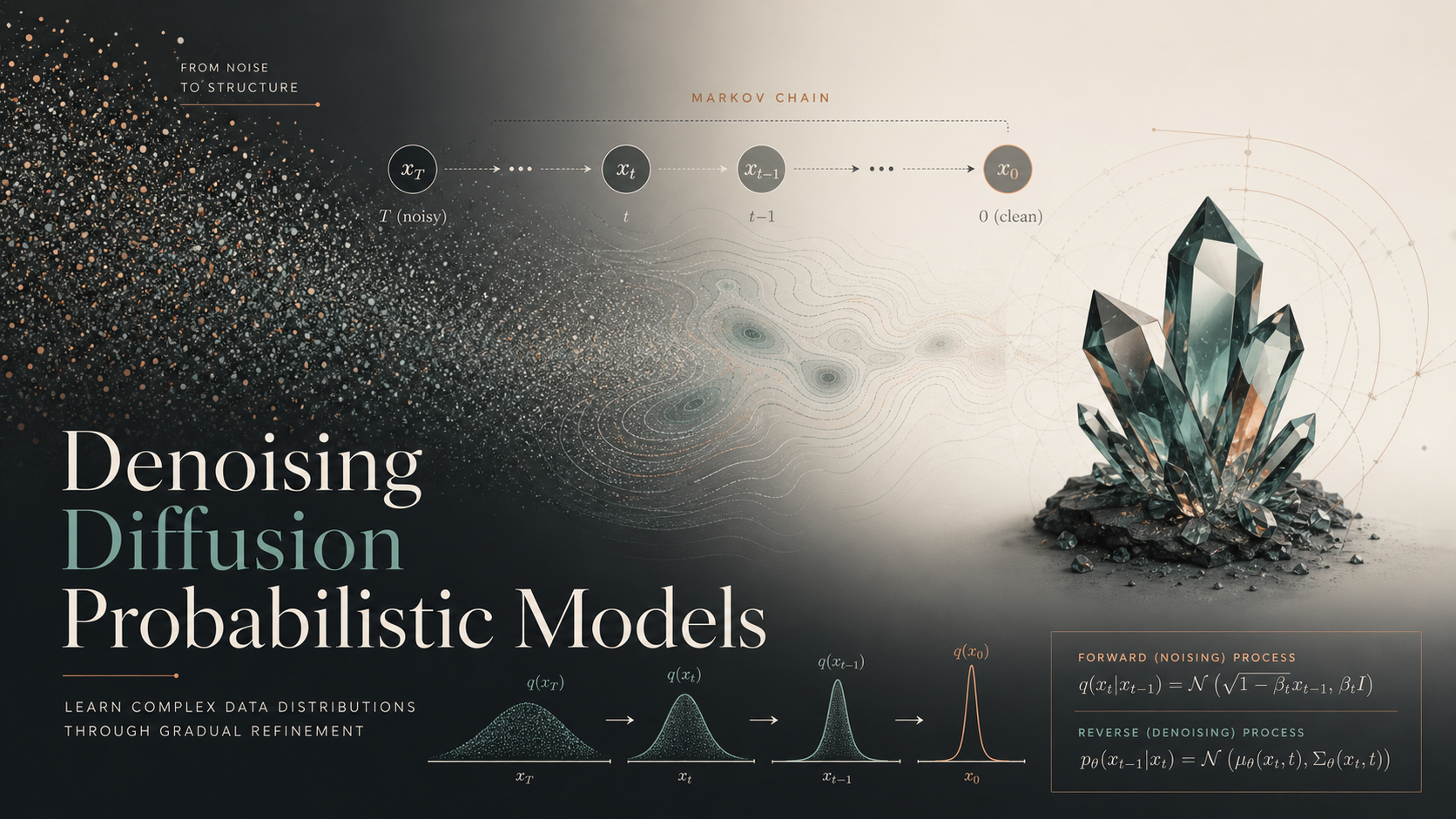
Paper: Jonathan Ho, Ajay Jain, Pieter Abbeel. Denoising Diffusion Probabilistic Models. NeurIPS 2020. arXiv: 2006.11239 · Code: hojonathanho/diffusion
This guide walks through the full technical content of the paper: the probabilistic setup, every derivation needed to arrive at the training objective, the training and sampling algorithms, the architecture, the experiments, and the paper’s interpretation of diffusion models as progressive lossy decoders.
Why this paper matters
Before DDPM, “diffusion probabilistic models” (Sohl-Dickstein et al., 2015) were a theoretically elegant but practically unproven idea: define a Markov chain that slowly destroys structure in data by adding noise, then learn to reverse it. GANs, VAEs, flows, and autoregressive models were all producing sharp samples; diffusion models were not known to be competitive.
Ho, Jain, and Abbeel’s contribution was to show that with the right parameterization, diffusion models generate CIFAR-10 samples with an Inception Score of 9.46 and an FID of 3.17 — beating essentially all published generative models on that benchmark at the time — and produce LSUN/CelebA-HQ 256×256 samples competitive with ProgressiveGAN. Just as importantly, they show that a particular parameterization choice makes the training objective equivalent to denoising score matching across multiple noise scales, unifying diffusion models with the score-based generative modeling line of work (Song & Ermon, 2019).
The price paid for this sample quality: DDPMs are not competitive on log-likelihood compared to autoregressive/flow models, and sampling requires a full sequential pass through hundreds or thousands of denoising steps (this second issue is what later work like DDIM and distillation methods addresses).
Setup: latent variable models with a fixed encoder
A diffusion model is a latent-variable model
\[p_\theta(\mathbf{x}_0) := \int p_\theta(\mathbf{x}_{0:T})\, d\mathbf{x}_{1:T}\]
where \(\mathbf{x}_1, \dots, \mathbf{x}_T\) are latents with the same dimensionality as the data \(\mathbf{x}_0 \sim q(\mathbf{x}_0)\). This is unlike a VAE, where the latent is lower-dimensional and the encoder is learned. Here:
- The approximate posterior \(q(\mathbf{x}_{1:T} \mid \mathbf{x}_0)\) — called the forward or diffusion process — is fixed (not learned) and is itself a Markov chain that gradually adds Gaussian noise according to a variance schedule \(\beta_1, \dots, \beta_T\).
- The reverse process \(p_\theta(\mathbf{x}_{0:T})\) is a learned Markov chain that starts at \(p(\mathbf{x}_T) = \mathcal{N}(\mathbf{x}_T; \mathbf{0}, \mathbf{I})\) and denoises step by step back to data.
Because both processes are Markov chains of conditional Gaussians, the whole model reduces to learning the mean (and optionally variance) of a Gaussian at every step — “a particularly simple neural network parameterization,” in the paper’s words.
The forward (diffusion) process
\[q(\mathbf{x}_{1:T} \mid \mathbf{x}_0) := \prod_{t=1}^{T} q(\mathbf{x}_t \mid \mathbf{x}_{t-1}), \qquad q(\mathbf{x}_t \mid \mathbf{x}_{t-1}) := \mathcal{N}\big(\mathbf{x}_t; \sqrt{1-\beta_t}\,\mathbf{x}_{t-1},\, \beta_t \mathbf{I}\big)\]
At each step, a small amount of Gaussian noise is added and the signal is slightly rescaled down. \(\beta_1, \dots, \beta_T\) is a fixed (not learned) variance schedule; in this paper it is a linear schedule from \(\beta_1 = 10^{-4}\) to \(\beta_T = 0.02\) with \(T = 1000\).
Closed-form marginal. Define \(\alpha_t := 1 - \beta_t\) and \(\bar\alpha_t := \prod_{s=1}^{t} \alpha_s\). Using the reparameterization trick and the fact that a sum of independent Gaussians is Gaussian, the forward process admits sampling \(\mathbf{x}_t\) at any timestep directly from \(\mathbf{x}_0\) in closed form, without stepping through the chain:
\[q(\mathbf{x}_t \mid \mathbf{x}_0) = \mathcal{N}\big(\mathbf{x}_t;\, \sqrt{\bar\alpha_t}\,\mathbf{x}_0,\, (1-\bar\alpha_t)\mathbf{I}\big)\]
Equivalently, with \(\boldsymbol\epsilon \sim \mathcal{N}(\mathbf{0}, \mathbf{I})\):
\[\mathbf{x}_t = \sqrt{\bar\alpha_t}\,\mathbf{x}_0 + \sqrt{1-\bar\alpha_t}\,\boldsymbol\epsilon\]
This identity is the workhorse of the entire paper — it lets training sample a random timestep \(t\) and jump straight to the noised image \(\mathbf{x}_t\), rather than simulating \(t\) sequential noising steps. As \(t \to T\), \(\bar\alpha_t \to 0\) and \(\mathbf{x}_T\) becomes (approximately) isotropic Gaussian noise, matching the prior \(p(\mathbf{x}_T)\).
The reverse process
\[p_\theta(\mathbf{x}_{0:T}) := p(\mathbf{x}_T) \prod_{t=1}^{T} p_\theta(\mathbf{x}_{t-1}\mid \mathbf{x}_t), \qquad p_\theta(\mathbf{x}_{t-1}\mid\mathbf{x}_t) := \mathcal{N}\big(\mathbf{x}_{t-1};\, \boldsymbol\mu_\theta(\mathbf{x}_t, t),\, \boldsymbol\Sigma_\theta(\mathbf{x}_t, t)\big)\]
A single neural network (conditioned on the timestep \(t\)) predicts the mean \(\boldsymbol\mu_\theta\) (and, in the simplest variant of the paper, the variance is fixed rather than learned — see Section 1.4). Sampling means starting from pure noise \(\mathbf{x}_T \sim \mathcal{N}(0, I)\) and iteratively drawing \(\mathbf{x}_{t-1} \sim p_\theta(\mathbf{x}_{t-1}\mid\mathbf{x}_t)\) down to \(\mathbf{x}_0\).
The diagram below is the paper’s Figure 2: the directed graphical model showing both processes on the same chain of variables. The forward process \(q\) moves left-to-right (adding noise, fixed, no learned parameters); the reverse process \(p_\theta\) moves right-to-left (removing noise, learned).
flowchart LR
    X0["x0 (data)"] -- "q(x1|x0)" --> X1["x1"]
    X1 -- "q(x2|x1)" --> X2["x2"]
    X2 -- "q(x3|x2)" --> Xdots["..."]
    Xdots -- "q(xT|xT-1)" --> XT["xT ~ N(0, I)"]

    XT -. "p_theta(xT-1|xT)" .-> Xdots
    Xdots -. "p_theta(x2|x3)" .-> X2
    X2 -. "p_theta(x1|x2)" .-> X1
    X1 -. "p_theta(x0|x1)" .-> X0

    classDef fwd fill:#e0ecff,stroke:#4472c4,color:#1f2937;
    class X0,X1,X2,Xdots,XT fwd
(Solid arrows: fixed forward diffusion \(q\), adding noise. Dashed arrows: learned reverse denoising \(p_\theta\), removing noise. This is a redrawing, in Mermaid, of the paper’s Figure 2 directed graphical model.)
Deriving the training objective
The variational bound
Since \(p_\theta(\mathbf{x}_0)\) requires an intractable integral, training proceeds by minimizing a variational bound on negative log-likelihood, exactly as in a VAE, using \(q\) as the fixed “encoder”:
\[\mathbb{E}[-\log p_\theta(\mathbf{x}_0)] \le \mathbb{E}_q\left[-\log \frac{p_\theta(\mathbf{x}_{0:T})}{q(\mathbf{x}_{1:T}\mid\mathbf{x}_0)}\right] =: L\]
Expanding this using the Markov structure of both chains and regrouping terms via Bayes’ rule (the standard DDPM/Sohl-Dickstein derivation) yields a sum of KL divergences between Gaussians, which are analytically tractable:
\[L = \underbrace{D_{KL}\big(q(\mathbf{x}_T\mid\mathbf{x}_0) \,\|\, p(\mathbf{x}_T)\big)}_{L_T} + \sum_{t=2}^{T} \underbrace{D_{KL}\big(q(\mathbf{x}_{t-1}\mid\mathbf{x}_t,\mathbf{x}_0) \,\|\, p_\theta(\mathbf{x}_{t-1}\mid\mathbf{x}_t)\big)}_{L_{t-1}} \;\underbrace{- \log p_\theta(\mathbf{x}_0\mid\mathbf{x}_1)}_{L_0}\]
- \(L_T\) has no learnable parameters (\(q\) is fixed and \(\beta\)’s are fixed constants), so it is a constant during training and can be ignored, provided \(\bar\alpha_T \approx 0\) so that \(q(\mathbf{x}_T\mid\mathbf{x}_0) \approx \mathcal{N}(0,I) = p(\mathbf{x}_T)\).
- \(L_{t-1}\) for \(t = 2, \dots, T\) are the terms that actually drive learning: each one matches the learned reverse step to the true forward posterior \(q(\mathbf{x}_{t-1}\mid\mathbf{x}_t,\mathbf{x}_0)\) — i.e. what the noising step “really” did, given that we know the clean image \(\mathbf{x}_0\).
- \(L_0\) is a separate discrete decoder term (see below) handling the final step from continuous \(\mathbf{x}_1\) back to discrete pixel values.
The tractable forward posterior
Because \(q\) is Gaussian and Markov, conditioning additionally on \(\mathbf{x}_0\) (using Bayes’ rule) gives another Gaussian in closed form:
\[q(\mathbf{x}_{t-1}\mid\mathbf{x}_t,\mathbf{x}_0) = \mathcal{N}\big(\mathbf{x}_{t-1};\, \tilde{\boldsymbol\mu}_t(\mathbf{x}_t,\mathbf{x}_0),\, \tilde\beta_t \mathbf{I}\big)\]
with
\[\tilde{\boldsymbol\mu}_t(\mathbf{x}_t,\mathbf{x}_0) = \frac{\sqrt{\bar\alpha_{t-1}}\,\beta_t}{1-\bar\alpha_t}\,\mathbf{x}_0 + \frac{\sqrt{\alpha_t}\,(1-\bar\alpha_{t-1})}{1-\bar\alpha_t}\,\mathbf{x}_t, \qquad \tilde\beta_t = \frac{1-\bar\alpha_{t-1}}{1-\bar\alpha_t}\,\beta_t\]
This \(q(\mathbf{x}_{t-1}\mid\mathbf{x}_t,\mathbf{x}_0)\) is exactly what \(p_\theta(\mathbf{x}_{t-1}\mid\mathbf{x}_t)\) is trained to approximate — except the network only has access to \(\mathbf{x}_t\) and \(t\), not the ground-truth \(\mathbf{x}_0\).
Reparameterizing the mean: predicting noise instead of the mean or the image
Since both \(q(\mathbf{x}_{t-1}\mid\mathbf{x}_t,\mathbf{x}_0)\) and \(p_\theta(\mathbf{x}_{t-1}\mid\mathbf{x}_t)\) are Gaussians, their KL divergence reduces to a squared difference of means (scaled by variance):
\[L_{t-1} = \mathbb{E}_q\left[\frac{1}{2\sigma_t^2}\left\| \tilde{\boldsymbol\mu}_t(\mathbf{x}_t,\mathbf{x}_0) - \boldsymbol\mu_\theta(\mathbf{x}_t,t) \right\|^2\right] + C\]
The paper’s key move: instead of directly predicting the mean, substitute the forward-process identity \(\mathbf{x}_0 = \frac{1}{\sqrt{\bar\alpha_t}}\big(\mathbf{x}_t - \sqrt{1-\bar\alpha_t}\,\boldsymbol\epsilon\big)\) into \(\tilde{\boldsymbol\mu}_t\). This shows that \(\tilde{\boldsymbol\mu}_t\) can be written purely as a function of \(\mathbf{x}_t\) and the noise \(\boldsymbol\epsilon\) that produced it:
\[\tilde{\boldsymbol\mu}_t(\mathbf{x}_t, \mathbf{x}_0) = \frac{1}{\sqrt{\alpha_t}}\left(\mathbf{x}_t - \frac{\beta_t}{\sqrt{1-\bar\alpha_t}}\,\boldsymbol\epsilon\right)\]
So instead of asking the network to predict the mean directly, we parameterize it to predict the noise \(\boldsymbol\epsilon\) that was added:
\[\boldsymbol\mu_\theta(\mathbf{x}_t, t) = \frac{1}{\sqrt{\alpha_t}}\left(\mathbf{x}_t - \frac{\beta_t}{\sqrt{1-\bar\alpha_t}}\,\boldsymbol\epsilon_\theta(\mathbf{x}_t, t)\right)\]
Plugging this back in, the loss term collapses to a simple noise-prediction MSE:
\[L_{t-1} = \mathbb{E}_{\mathbf{x}_0,\boldsymbol\epsilon}\left[\frac{\beta_t^2}{2\sigma_t^2 \alpha_t (1-\bar\alpha_t)} \left\| \boldsymbol\epsilon - \boldsymbol\epsilon_\theta\big(\sqrt{\bar\alpha_t}\,\mathbf{x}_0 + \sqrt{1-\bar\alpha_t}\,\boldsymbol\epsilon,\; t\big) \right\|^2 \right]\]
Intuitively: the network is a denoiser. Given a noisy image \(\mathbf{x}_t\) and the timestep \(t\), it predicts the noise vector that was mixed in, and the reverse step subtracts a scaled version of that prediction.
For the variance \(\boldsymbol\Sigma_\theta(\mathbf{x}_t,t) = \sigma_t^2\mathbf{I}\), the paper fixes it (untrained) to either \(\sigma_t^2 = \beta_t\) (matching the case where \(\mathbf{x}_0 \sim \mathcal{N}(0,I)\)) or \(\sigma_t^2 = \tilde\beta_t\) (matching a deterministic \(\mathbf{x}_0\)); both gave similar results experimentally.
The final decoder term \(L_0\)
Images are stored as integers in \(\{0, \dots, 255\}\), linearly scaled to \([-1, 1]\). To go from the continuous Gaussian model \(p_\theta(\mathbf{x}_0\mid\mathbf{x}_1)\) back to a distribution over discrete pixel values, the paper derives an independent discrete decoder for each pixel/channel: it integrates the Gaussian density \(\mathcal{N}(\mathbf{x}_0; \boldsymbol\mu_\theta(\mathbf{x}_1,1), \sigma_1^2\mathbf{I})\) over the small interval around each discrete pixel value, ensuring the model’s log-likelihood is a fair comparison against other likelihood-based models operating on discrete data (similar in spirit to PixelCNN++’s discretized logistic mixture decoder).
The simplified training objective, \(L_\text{simple}\)
The weighting term \(\frac{\beta_t^2}{2\sigma_t^2\alpha_t(1-\bar\alpha_t)}\) in front of the MSE above down-weights the loss for small \(t\) (where noise is barely perceptible) relative to large \(t\). The paper finds that dropping this weighting — training on the plain, unweighted noise-prediction MSE — produces a more effective training target that emphasizes harder, higher-noise denoising tasks and empirically improves sample quality (at the cost of the resulting objective no longer being a valid bound on log-likelihood):
\[L_\text{simple}(\theta) := \mathbb{E}_{t \sim \mathcal U(1,T),\, \mathbf{x}_0,\, \boldsymbol\epsilon \sim \mathcal{N}(0,I)}\Big[\big\| \boldsymbol\epsilon - \boldsymbol\epsilon_\theta(\sqrt{\bar\alpha_t}\,\mathbf{x}_0 + \sqrt{1-\bar\alpha_t}\,\boldsymbol\epsilon,\; t) \big\|^2\Big]\]
This is the loss actually used to train the best models in the paper. It is remarkably close to the denoising score-matching objectives used in score-based generative models (see below), which is the connection the paper highlights as one of its main contributions.
Training and sampling algorithms
Algorithm 1 — Training
repeat
    x_0 ~ q(x_0)                                   # sample a real image
    t ~ Uniform({1, ..., T})                       # sample a random timestep
    epsilon ~ N(0, I)                              # sample noise
    take a gradient descent step on
        grad_theta || epsilon - epsilon_theta( sqrt(abar_t) x_0 + sqrt(1-abar_t) epsilon,  t ) ||^2
until converged
Algorithm 2 — Sampling
x_T ~ N(0, I)
for t = T, ..., 1:
    z ~ N(0, I)   if t > 1,   else z = 0
    x_{t-1} = (1/sqrt(alpha_t)) ( x_t - (beta_t/sqrt(1-abar_t)) epsilon_theta(x_t, t) )  +  sigma_t z
return x_0
Training is a single forward pass per step (efficient — no need to unroll the chain), but sampling is inherently sequential: generating one image requires \(T\) (up to 1000) full network evaluations, each depending on the previous. This asymmetry — cheap training, expensive sampling — is the central practical drawback of DDPMs and the main target of later speedups (e.g. DDIM’s non-Markovian samplers, distillation, and fewer-step schedules).
The following flowchart summarizes the sampling loop end to end:
flowchart TD
    Start(["Sample x_T ~ N(0, I)"]) --> Loop{"t = T ... 1"}
    Loop --> Predict["Network predicts noise: epsilon_theta(x_t, t)"]
    Predict --> Mean["Compute mean mu:
    mu = (1/sqrt(alpha_t)) * (x_t - beta_t/sqrt(1-abar_t) * epsilon_theta)"]
    Mean --> Check{"t > 1 ?"}
    Check -- yes --> AddNoise["x_(t-1) = mu + sigma_t * z,  z ~ N(0,I)"]
    Check -- no --> NoNoise["x_0 = mu  (no noise added)"]
    AddNoise --> Loop
    NoNoise --> Done(["Return x_0 (generated image)"])
Connection to denoising score matching and Langevin dynamics
A separate line of work (score matching, Song & Ermon 2019) trains a network \(\mathbf{s}_\theta(\mathbf{x}, \sigma)\) to estimate the score \(\nabla_\mathbf{x} \log q(\mathbf{x})\) of data perturbed by noise level \(\sigma\), then generates samples via annealed Langevin dynamics: iteratively nudging a sample in the direction of increasing log-density, with noise levels annealed from large to small.
The paper observes that the noise-prediction network \(\boldsymbol\epsilon_\theta\) trained with \(L_\text{simple}\) is, up to a constant scaling factor, estimating the score of the noised data distribution:
\[\mathbf{s}_\theta(\mathbf{x}_t, t) \approx -\frac{\boldsymbol\epsilon_\theta(\mathbf{x}_t,t)}{\sqrt{1-\bar\alpha_t}}\]
and the reverse sampling update in Algorithm 2 is structurally identical to a step of Langevin dynamics using this score estimate, with the \(T\) diffusion noise levels playing the role of the annealed noise schedule. This means DDPM training is, in effect, simultaneously training a denoising autoencoder at every noise scale \(t = 1,\dots,T\) and generating samples via annealed Langevin-like updates — two previously separate ideas (diffusion models and score matching) turn out to be two views of the same objective. The paper considers this equivalence one of its primary contributions, not just an implementation detail, because the best empirical results come precisely from the parameterization that makes this connection exact.
Model architecture
The reverse-process network \(\boldsymbol\epsilon_\theta(\mathbf{x}_t, t)\) is a single U-Net shared across all timesteps, conditioned on \(t\):
- Backbone: a U-Net in the style of PixelCNN++’s Wide ResNet, adapted with group normalization in place of weight normalization.
- Multi-resolution structure: downsampling then upsampling convolutional stages (encoder–decoder with skip connections), each resolution level built from residual blocks.
- Self-attention: attention blocks are inserted at the 16×16 feature-map resolution (between convolutional residual blocks), letting the model capture long-range spatial dependence in addition to local convolutional structure.
- Timestep conditioning: the timestep \(t\) is embedded using sinusoidal position embeddings (the same construction used for positional encoding in Transformers) and injected into every residual block, so a single network can specialize its denoising behavior to the current noise level.
- Weight sharing across resolutions: because \(\mathbf{x}_t\) always has the same dimensionality as \(\mathbf{x}_0\), the same network architecture handles every timestep — there is no need for \(T\) separate networks.
Key hyperparameters used in the paper:
| Setting | Value |
|---|---|
| Diffusion steps \(T\) | 1000 |
| Variance schedule \(\beta_t\) | linear, \(\beta_1 = 10^{-4} \to \beta_T = 0.02\) |
| Optimizer | Adam |
| Data scaling | pixels linearly scaled to \([-1, 1]\) |
| Regularization (CIFAR-10) | dropout, plus random horizontal flips |
| Weight averaging | exponential moving average (EMA) of model weights used for sampling/evaluation |
| Datasets | CIFAR-10 (32×32), LSUN Bedroom/Church (256×256), CelebA-HQ (256×256) |
Experiments and results
Sample quality
On unconditional CIFAR-10, the paper reports (Table 1 of the paper):
| Model variant | Inception Score ↑ | FID ↓ |
|---|---|---|
| DDPM, fixed variance (\(\sigma_t^2 = \beta_t\)), \(L_\text{simple}\) objective (best) | 9.46 | 3.17 |
At the time of publication this FID was state-of-the-art among unconditional CIFAR-10 models, and the reported FID against the CIFAR-10 test set (rather than train) is 5.24 — still competitive with training-set FID numbers reported for many prior models. On 256×256 LSUN Church/Bedroom and CelebA-HQ, the paper reports sample quality “similar to ProgressiveGAN,” a strong GAN-based baseline for high-resolution unconditional generation at the time.
Reverse-process parameterization and objective ablation
The paper systematically ablates:
- What the network predicts — the raw mean \(\boldsymbol\mu_\theta\), the clean image \(\mathbf{x}_0\), or the noise \(\boldsymbol\epsilon\).
- Whether \(\boldsymbol\Sigma_\theta\) is fixed or learned.
- Whether the loss is the properly weighted variational bound \(L_\text{vlb}\) or the unweighted \(L_\text{simple}\).
The clear winner for sample quality is \(\boldsymbol\epsilon\)-prediction with the unweighted \(L_\text{simple}\) loss and fixed variance — this is the configuration used for the headline CIFAR-10/LSUN/CelebA-HQ results. Predicting \(\mathbf{x}_0\) directly (rather than \(\boldsymbol\epsilon\)) trains far less stably and produces noticeably worse samples, especially early in training. Training with the fully weighted \(L_\text{vlb}\) gives better log-likelihoods (as expected, since it is the actual variational bound) but worse perceptual sample quality than \(L_\text{simple}\) — a quality/likelihood trade-off that the paper flags as an open question.
Likelihood / lossless codelength
Despite excellent samples, DDPM’s negative log-likelihood on CIFAR-10 (≤ 3.75 bits/dim under the best variant) is not competitive with dedicated likelihood-based models such as autoregressive PixelCNN-family models or normalizing flows, which achieve markedly lower bits/dim. The paper investigates why using a rate–distortion analysis: it decomposes the lossless codelength into contributions from each reverse step and plots how quickly image distortion (reconstruction quality) improves as more rate (bits) is spent decoding. This shows that the overwhelming majority of the model’s bits are spent describing imperceptible, high-frequency image details, while the perceptually important large-scale structure of the image is captured using only a small fraction of the total codelength. This explains the apparent paradox: a model can produce excellent-looking samples while still not achieving a good likelihood score, because likelihood cares equally about every bit, including bits humans cannot perceive.
Progressive generation as generalized autoregressive decoding
Because sampling proceeds through \(\mathbf{x}_T \to \mathbf{x}_{T-1} \to \dots \to \mathbf{x}_0\), one can inspect intermediate reconstructions \(\hat{\mathbf{x}}_0\) predicted at each step along the way. The paper shows that this progressive decoding reveals large-scale image structure (rough shapes, layout) emerging first, with fine detail filled in only at the final steps — analogous to autoregressive image models decoding pixel-by-pixel, except that DDPM’s implicit “ordering” of information is over spatial frequency / scale rather than a fixed raster-scan pixel order, which the authors argue is a strict generalization of what autoregressive decoding can express.
Interpolation
The paper also demonstrates latent-space interpolation: encode two real images to a shared intermediate noise level \(\mathbf{x}_t\) (via the forward process), linearly interpolate the two noised latents, and run the reverse process back down to \(t=0\). This produces smooth, semantically plausible interpolations between the two source images, showing that intermediate diffusion latents encode meaningful structure rather than being pure noise.
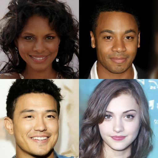
The paper contains multiple figures composed of actual generated image grids (unconditional CIFAR-10/CelebA-HQ/LSUN samples, progressive-generation image sequences, and interpolation grids) rather than schematic diagrams. These are best viewed directly in the source rather than reproduced as text; see the original paper — arXiv:2006.11239 (PDF) — Figure 1 (CelebA-HQ / CIFAR-10 samples), and the additional sample and progressive-generation figures in Sections 4 and Appendix. One figure asset is directly linkable:
Limitations and legacy
- Sampling cost. \(T=1000\) sequential network evaluations per sample is orders of magnitude slower than a single GAN forward pass. This motivated a large body of follow-up work on faster samplers (DDIM, samplers based on SDE/ODE solvers, distillation).
- Likelihood vs. sample quality trade-off. The best-sounding objective for samples (\(L_\text{simple}\)) is not the best for likelihood (\(L_\text{vlb}\)), and the paper leaves reconciling this as an open problem — later work (e.g. “Improved DDPM,” Nichol & Dhariwal 2021) directly addresses learned variances and hybrid objectives to close this gap.
- Fixed, hand-designed variance schedule. \(\beta_t\) is fixed and linear; later work learns or otherwise improves the noise schedule.
- Legacy. This paper, together with concurrent score-based generative modeling work, is the direct ancestor of the modern text-to-image diffusion pipeline (GLIDE, DALL·E 2, Imagen, Stable Diffusion), all of which reuse the same forward/reverse Gaussian diffusion formalism and \(\boldsymbol\epsilon\)-prediction training objective derived here, typically combined with classifier(-free) guidance and latent-space diffusion for efficiency.
Notation reference
| Symbol | Meaning |
|---|---|
| \(\mathbf{x}_0\) | a real data sample (e.g. an image) |
| \(\mathbf{x}_1, \dots, \mathbf{x}_T\) | latents of the same dimensionality as \(\mathbf{x}_0\), increasingly noisy |
| \(T\) | number of diffusion steps (1000 in this paper) |
| \(\beta_t\) | forward-process noise variance added at step \(t\) (fixed schedule) |
| \(\alpha_t := 1-\beta_t\) | signal-retention factor at step \(t\) |
| \(\bar\alpha_t := \prod_{s=1}^t \alpha_s\) | cumulative signal-retention factor from \(0\) to \(t\) |
| \(q(\cdot)\) | fixed forward (noising) process |
| \(p_\theta(\cdot)\) | learned reverse (denoising) process |
| \(\boldsymbol\epsilon_\theta(\mathbf{x}_t, t)\) | neural network predicting the noise added to produce \(\mathbf{x}_t\) |
| \(\boldsymbol\mu_\theta, \boldsymbol\Sigma_\theta\) | mean / covariance of the learned reverse Gaussian at step \(t\) |
| \(\tilde{\boldsymbol\mu}_t, \tilde\beta_t\) | mean / variance of the tractable forward posterior \(q(\mathbf{x}_{t-1}\mid \mathbf{x}_t,\mathbf{x}_0)\) |
| \(L_\text{vlb}\) | full weighted variational bound on negative log-likelihood |
| \(L_\text{simple}\) | unweighted noise-prediction MSE used in practice |
References
- Sohl-Dickstein, J., Weiss, E., Maheswaranathan, N., & Ganguli, S. (2015). Deep Unsupervised Learning using Nonequilibrium Thermodynamics.
- Song, Y., & Ermon, S. (2019). Generative Modeling by Estimating Gradients of the Data Distribution.
- Salimans, T., Karpathy, A., Chen, X., & Kingma, D. P. (2017). PixelCNN++: Improving the PixelCNN with Discretized Logistic Mixture Likelihood and Other Modifications.
- Kingma, D. P., & Ba, J. (2015). Adam: A Method for Stochastic Optimization.
- Karras, T., Aila, T., Laine, S., & Lehtinen, J. (2018). Progressive Growing of GANs for Improved Quality, Stability, and Variation (ProgressiveGAN — the sample-quality baseline used for LSUN/CelebA-HQ comparisons).
(Full reference list: see the original paper.)