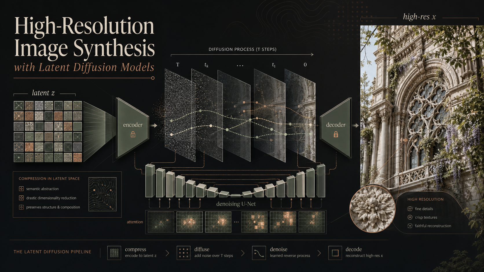
This is the paper that introduced Latent Diffusion Models (LDMs) — the architecture that underlies Stable Diffusion. Its core trick is deceptively simple: instead of running a diffusion model directly on RGB pixels, first compress the image into a small, perceptually equivalent latent space with an autoencoder, and run the (expensive, iterative) diffusion process there instead. This guide focuses on how and why that works, walking through the method in detail, with a lighter pass over the experimental results.
Paper: Rombach, Blattmann, Lorenz, Esser, Ommer (2021/2022). High-Resolution Image Synthesis with Latent Diffusion Models. CVPR 2022. arXiv:2112.10752
1. Why this paper exists
Diffusion models (DMs) had, by late 2021, become the state of the art for image synthesis — better mode coverage than GANs, no adversarial training instability, and strong likelihood-based density estimation. But they had a brutal cost problem:
- Training a powerful pixel-space DM could take 150–1000 V100 GPU-days.
- Generating 50,000 samples could take ~5 days on a single A100, because sampling requires many sequential forward passes of a large neural network.
The root cause is that DMs are likelihood-based models, and likelihood-based training is “mode-covering”: it spends a disproportionate amount of model capacity and compute on modeling imperceptible, high-frequency pixel details that contribute almost nothing to how an image looks to a human. Every one of those denoising steps still has to run over the full, high-dimensional pixel grid.
The authors’ insight is that image “information content” naturally splits into two regimes:
- Perceptual compression — removing high-frequency detail that a human wouldn’t notice is missing. This is what a good autoencoder or JPEG-style codec does.
- Semantic compression — learning the actual conceptual/semantic composition of the data. This is the hard generative modeling problem that diffusion models are good at.
Most of a pixel-space DM’s compute is wasted re-deriving perceptual compression that a much cheaper, non-iterative model could have done once, up front. So: separate the two stages. Train an autoencoder once to handle perceptual compression, then train the diffusion model entirely inside that compressed latent space, where it only has to worry about semantics.
flowchart LR
    subgraph S1["Stage 1 — trained once"]
        A[Pixel-space image] -->|"perceptual\ncompression"| B["Latent code z\n(small, smooth space)"]
    end
    subgraph S2["Stage 2 — the actual generative model"]
        B -->|"diffusion process\n(semantic compression)"| C["Denoised latent z₀"]
    end
    C -->|decode| D["Reconstructed / generated image"]

    style S1 fill:#eef,stroke:#446
    style S2 fill:#efe,stroke:#464
This separation is the entire idea of the paper. Everything else — the autoencoder design, the diffusion loss, the UNet, the cross-attention conditioning — is in service of making that separation work well.
2. Perceptual image compression (Stage 1: the autoencoder)
The first stage is an autoencoder \((\mathcal{E}, \mathcal{D})\) trained independently of the diffusion model, once, and then reused for many downstream diffusion models and tasks.
Given an image \(x \in \mathbb{R}^{H\times W\times 3}\):
- The encoder maps it to a latent \(z = \mathcal{E}(x)\).
- The decoder reconstructs it: \(\tilde{x} = \mathcal{D}(z) = \mathcal{D}(\mathcal{E}(x))\).
- \(z \in \mathbb{R}^{h \times w \times c}\), where the encoder downsamples spatially by a factor \(f = H/h = W/w\), with \(f = 2^m\) for various \(m\).
Two design choices matter a great deal here:
Loss function. Rather than training with a plain pixel-space \(L_1\)/\(L_2\) reconstruction loss (which produces blurry reconstructions because it’s satisfied by “safe,” averaged pixel values), the autoencoder uses a combination of a perceptual loss and a patch-based adversarial objective. This keeps reconstructions on the manifold of realistic images and enforces local realism, rather than optimizing a pixel-wise metric that doesn’t correlate well with perceived quality.
Regularizing the latent space. An unconstrained autoencoder latent space can have arbitrarily high variance, which is a bad target for a diffusion model to learn (it needs some regularity to interpolate/denoise sensibly). Two regularization schemes are tried:
- KL-reg.: a small KL penalty pulling the learned latent distribution toward a standard normal, à la a VAE.
- VQ-reg.: a vector-quantization layer, absorbed into the decoder — effectively a VQGAN, but where the diffusion model (not an autoregressive transformer) will model the prior over the latent.
Crucially, because the downstream diffusion model is a convolutional UNet that can exploit the 2D spatial structure of \(z\), this compression can stay mild — unlike prior two-stage approaches (VQGAN + autoregressive transformer) that needed to compress very aggressively (often flattening the latent into a 1D sequence) to keep the downstream autoregressive model computationally tractable. Keeping the latent 2D and only mildly compressed is what allows LDMs to get near-lossless reconstructions while still slashing computational cost — this is exactly the trade-off visualized in Figure 1 of the paper, where the LDM’s higher downsampling factor \(f{=}4\) still reconstructs images far more faithfully (PSNR 27.4, R-FID 0.58) than DALL·E’s discrete VAE at \(f{=}8\) (PSNR 22.8, R-FID 32.01) or the original VQGAN at \(f{=}16\) (PSNR 19.9, R-FID 4.98).
(This is one of eight reconstruction comparisons in the paper’s Figure 1; see the full paper for all of them.)

3. Latent Diffusion Models (Stage 2: the actual generative model)
3.1 A quick refresher on diffusion models
A standard denoising diffusion probabilistic model learns \(p(x)\) by learning to reverse a fixed-length (\(T\)-step) Markov chain that gradually adds Gaussian noise to data. In practice this reduces to training a sequence of denoising autoencoders \(\epsilon_\theta(x_t, t)\), \(t = 1 \ldots T\), each of which is trained to predict the noise \(\epsilon\) that was added to produce the noisy sample \(x_t\) from the clean data \(x\). The (simplified, reweighted) training objective is:
\[ L_{DM} = \mathbb{E}_{x,\,\epsilon \sim \mathcal{N}(0,1),\,t}\Big[\|\epsilon - \epsilon_\theta(x_t, t)\|_2^2\Big] \tag{1} \]
with \(t\) sampled uniformly from \(\{1, \ldots, T\}\). This is normally evaluated and optimized directly on RGB pixels \(x\) — which is the expensive part.
3.2 Moving the diffusion process into latent space
Once the perceptual autoencoder \((\mathcal{E}, \mathcal{D})\) from Section 2 is trained and frozen, LDMs simply replace \(x\) with \(z = \mathcal{E}(x)\) everywhere in the diffusion objective:
\[ L_{LDM} := \mathbb{E}_{\mathcal{E}(x),\,\epsilon \sim \mathcal{N}(0,1),\,t}\Big[\|\epsilon - \epsilon_\theta(z_t, t)\|_2^2\Big] \tag{2} \]
The denoising network \(\epsilon_\theta(\circ, t)\) is a time-conditional UNet, now built primarily from 2D convolutional layers operating on the small \(h \times w \times c\) latent grid instead of the full \(H \times W \times 3\) pixel grid. Because the forward (noising) process is fixed and closed-form, \(z_t\) can be computed cheaply from \(\mathcal{E}(x)\) during training — there’s no need to run the decoder at every training step. At sampling time, you run the reverse diffusion process entirely in latent space to get a sample \(z \sim p(z)\), and only decode once at the very end via \(\mathcal{D}\).
This is the entire computational win: the same UNet architecture and the same number of diffusion steps now operate on a grid that might be, say, \(32\times32\times4\) instead of \(256\times256\times3\) — dramatically cutting both training FLOPs and sampling latency, since sampling requires many sequential evaluations of \(\epsilon_\theta\).
flowchart TB
    subgraph Training
        direction LR
        X["image x"] -->|"frozen encoder ℰ"| Z0["z = ℰ(x)"]
        Z0 -->|"add noise (forward process)"| ZT["z_t"]
        ZT -->|"UNet ε_θ(z_t, t)"| EPS["predicted noise ε̂"]
        EPS -->|"compare to true ε"| LOSS["L_LDM loss"]
    end
flowchart LR
    N["z_T ~ N(0, I)\n(pure noise latent)"] -->|"reverse diffusion,\nT denoising steps\nwith ε_θ"| Z0["z_0\n(denoised latent)"]
    Z0 -->|"frozen decoder 𝒟"| IMG["generated image"]
3.3 Conditioning mechanisms: turning LDMs into controllable generators
An unconditional diffusion model just samples “some image from the training distribution.” To make it useful — text-to-image, layout-to-image, class-conditional, super-resolution, inpainting — the model needs to condition on side information \(y\). The paper handles this in two ways depending on the task:
1. Spatial concatenation. For densely-aligned conditioning signals that live in the same spatial grid as the image (a low-resolution image for super-resolution, a semantic segmentation map, a masked image for inpainting), the conditioning signal is simply concatenated channel-wise to the UNet’s input. This is cheap and works well precisely because the signal is already spatially aligned with \(z_t\).
2. Cross-attention, for general/unaligned conditioning. For anything that isn’t naturally a spatial map — most importantly, free-form text — the paper augments the UNet with cross-attention layers. A domain-specific encoder \(\tau_\theta\) (e.g. a transformer over BERT-tokenized text) projects the conditioning input \(y\) into an intermediate representation \(\tau_\theta(y) \in \mathbb{R}^{M \times d_\tau}\). This is then fed into the UNet’s intermediate layers via standard multi-head cross-attention:
\[ \text{Attention}(Q, K, V) = \text{softmax}\!\left(\frac{QK^T}{\sqrt{d}}\right)\cdot V \]
\[ Q = W_Q^{(i)} \cdot \varphi_i(z_t), \quad K = W_K^{(i)} \cdot \tau_\theta(y), \quad V = W_V^{(i)} \cdot \tau_\theta(y) \]
where \(\varphi_i(z_t) \in \mathbb{R}^{N \times d_\epsilon^i}\) is a flattened intermediate UNet feature map, and \(W_Q^{(i)}, W_K^{(i)}, W_V^{(i)}\) are learned projection matrices at that layer. In plain terms: the image latent’s spatial features (as queries) attend over the tokens of the conditioning representation (as keys/values) — exactly the mechanism transformers use for cross-modal attention, just injected into a convolutional UNet at multiple resolutions.
Both \(\tau_\theta\) and \(\epsilon_\theta\) are trained jointly, end to end, by minimizing the conditional variant of the LDM loss:
\[ L_{LDM} := \mathbb{E}_{\mathcal{E}(x),\,y,\,\epsilon\sim\mathcal{N}(0,1),\,t}\Big[\|\epsilon - \epsilon_\theta(z_t, t, \tau_\theta(y))\|_2^2\Big] \tag{3} \]
This is the paper’s Figure 3, redrawn below as a flowchart: an image is compressed to a latent, noised, and denoised by a UNet that at several resolutions either (a) concatenates spatially-aligned conditioning directly into its input/feature maps, or (b) attends over a conditioning encoder’s output via cross-attention.
flowchart TB
    IMG["Input image x\n(pixel space)"] -->|"encoder ℰ"| Z["latent z"]
    Z --> NOISE["diffusion process\n(forward: add noise)"]
    NOISE --> ZT["noisy latent z_t"]

    subgraph UNET["Denoising UNet ε_θ(z_t, t, ·)"]
        direction TB
        CONV["Conv / ResNet blocks\n(multi-resolution)"]
        XATTN["Cross-attention layers\nQ from image features\nK, V from τ_θ(y)"]
        CONV <--> XATTN
    end

    ZT --> UNET

    YTEXT["Conditioning y\n(text / class / layout / etc.)"] -->|"domain encoder τ_θ\n(e.g. transformer)"| TAU["τ_θ(y)"]
    TAU --> XATTN

    YSPATIAL["Spatially-aligned conditioning\n(low-res image, mask, semantic map)"] -->|"concatenate channel-wise"| CONV

    UNET --> ZPRED["predicted / denoised latent"]
    ZPRED -->|"decoder 𝒟"| OUT["output image"]

    style UNET fill:#eef,stroke:#446
The cross-attention route is what lets the same architecture handle text-to-image, class-conditional, and layout-to-image generation just by swapping out \(\tau_\theta\) and the training data — no task-specific architecture needed. The concatenation route is what lets the model be applied convolutionally to render images much larger than it was trained on (Section 5 below), since concatenation-based conditioning has no fixed sequence length the way cross-attention over a fixed set of tokens does.
4. Experiments (condensed)
The paper runs a large experimental sweep; here are the headline findings.
Finding the right compression factor. The authors sweep the downsampling factor \(f \in \{1, 2, 4, 8, 16, 32\}\) (calling the pixel-space case, \(f{=}1\), “LDM-1”). Small \(f\) (little compression) makes training slow, because the diffusion model is still mostly doing perceptual compression itself. Large \(f\) (aggressive compression) causes fidelity to plateau early, because too much information is lost in Stage 1 before the diffusion model ever sees the data. LDM-4 and LDM-8 hit the sweet spot — after 2M training steps, LDM-8 shows a 38-point FID improvement over pixel-based LDM-1, while sampling substantially faster.
Unconditional image generation. Trained on CelebA-HQ, FFHQ, LSUN-Churches, and LSUN-Bedrooms at 256×256, LDMs set a new state-of-the-art FID of 5.11 on CelebA-HQ, beating both prior likelihood-based models and GANs, and consistently improve Precision/Recall over GAN baselines — evidence of the better mode coverage that comes from likelihood-based training.
Text-to-image synthesis. A 1.45B-parameter KL-regularized LDM (BERT tokenizer + transformer as \(\tau_\theta\)), trained on LAION-400M, is evaluated on MS-COCO. With classifier-free guidance, it becomes competitive with contemporaneous state-of-the-art autoregressive (Make-A-Scene) and diffusion (GLIDE) text-to-image models, while using substantially fewer parameters than either.
Class-conditional ImageNet. LDM-4 with classifier-free guidance beats ADM (the prior best diffusion model for this task) while using roughly half the parameters and about 4× less training compute.
Convolutional sampling beyond 256². Because spatially-aligned conditioning is injected by concatenation rather than a fixed-length attention context, an LDM trained at 256×256 can be applied convolutionally at inference time to synthesize much larger, spatially coherent images (up to ~1024² in some settings) — demonstrated on semantic-layout-to-landscape synthesis at 512×1024.
Super-resolution & inpainting. LDMs trained for 4× super-resolution (conditioning by concatenating a low-res image) are competitive with the specialized SR3 diffusion model, and LDM-based inpainting sets a new state-of-the-art FID versus the specialized LaMa architecture, while human raters preferred LDM inpainting results in a user study.
Across nearly every task, the consistent story is: comparable or better sample quality than pixel-space diffusion models or GANs, at a fraction of the training and sampling compute.
6. Why this paper mattered
Conceptually, the contribution isn’t a new generative modeling principle — it’s a systems-level re-architecture: decouple “make it look real at the pixel level” (autoencoder, trained once, fast) from “make it semantically coherent/controllable” (diffusion, iterative, now much cheaper because it runs on a small latent grid), and glue them together with a general-purpose cross-attention conditioning mechanism that works for text, class labels, layouts, or anything else you can encode into tokens.
That combination — cheap latent-space diffusion + flexible cross-attention conditioning — is exactly the recipe later scaled up (with a larger UNet, a bigger text encoder, and web-scale text-image data) to become Stable Diffusion, which is why this paper is often cited as the latent diffusion / Stable Diffusion paper even though the original public release came somewhat later.
Key equations at a glance
| # | Equation | What it is |
|---|---|---|
| 1 | \(L_{DM} = \mathbb{E}_{x,\epsilon\sim\mathcal{N}(0,1),t}\big[\lVert\epsilon-\epsilon_\theta(x_t,t)\rVert_2^2\big]\) | Standard pixel-space diffusion loss |
| 2 | \(L_{LDM} := \mathbb{E}_{\mathcal{E}(x),\epsilon\sim\mathcal{N}(0,1),t}\big[\lVert\epsilon-\epsilon_\theta(z_t,t)\rVert_2^2\big]\) | Same loss, moved into latent space |
| — | \(\text{Attention}(Q,K,V)=\text{softmax}\!\left(\frac{QK^T}{\sqrt d}\right)\cdot V\) | Cross-attention used for conditioning |
| 3 | \(L_{LDM} := \mathbb{E}_{\mathcal{E}(x),y,\epsilon\sim\mathcal{N}(0,1),t}\big[\lVert\epsilon-\epsilon_\theta(z_t,t,\tau_\theta(y))\rVert_2^2\big]\) | Conditional LDM loss with cross-attention conditioning |
Source: Rombach et al., “High-Resolution Image Synthesis with Latent Diffusion Models,” CVPR 2022 / arXiv:2112.10752. Code: github.com/CompVis/latent-diffusion.